Intercomparison of XH₂O Data from the GOSAT TANSO-FTS (TIR and SWIR) and Ground-Based FTS Measurements: Impact of the Spatial Variability of XH₂O on the Intercomparison

Abstract

Spatial and temporal variability of atmospheric water vapor (H₂O) is extremely high, and therefore it is difficult to accurately evaluate the measurement precision of H₂O data by a simple comparison between the data derived from two different instruments. We determined the measurement precisions of column-averaged dry-air mole fractions of H₂O (XH₂O) retrieved independently from spectral radiances in the thermal infrared (TIR) and the short-wavelength infrared (SWIR) regions measured using a Thermal And Near-infrared Sensor for carbon Observation-Fourier Transform Spectrometer (TANSO-FTS) onboard the Greenhouse gases Observing SATellite (GOSAT), by an intercomparison between the two TANSO-FTS XH₂O data products and the ground-based FTS XH₂O data. Furthermore, the spatial variability of XH₂O was also estimated in the intercomparison process. Mutually coincident XH₂O data above land for the period ranging from April 2009 to May 2014 were intercompared with different spatial coincidence criteria. We found that the precisions of the TANSO-FTS TIR and TANSO-FTS SWIR XH₂O were 7.3%–7.7% and 3.5%–4.5%, respectively, and that the spatial variability of XH₂O was 6.7% within a radius of 50 km and 18.5% within a radius of 200 km. These results demonstrate that, in order to accurately evaluate the measurement precision of XH₂O, it is necessary to set more rigorous spatial coincidence criteria or to take into account the spatial variability of XH₂O as derived in the present study.

1. Introduction

Water vapor (H₂O) is the most abundant and variable natural greenhouse gas in the Earth’s atmosphere. It also plays an essential role in the global hydrological cycle via the formation of clouds and precipitation, and thereby contributes significantly to weather and climate. Monitoring the distribution, variability, and long-term changes in water vapor is critical to understanding the hydrological cycle, radiative budget, and climate change. The integrated water vapor (IWV) and H₂O profile have been measured by both in situ and remote sensing methods [1], and their data have been utilized for data assimilation in numerical weather prediction and trend analysis.

Given that there is a possibility of systematic bias in measurements, the bias should be corrected before the data assimilation, while a relative precision of the data is required in the data assimilation process. Intercomparison of IWV derived from different techniques or instruments is a commonly used method for assessing the bias and relative precision of the data [2]. The standard deviation of the mean difference between the IWV, which is obtained from the intercomparison, includes the spatial and temporal representativeness (variability) and the effect of difference in the vertical resolution between the two measurements, in addition to the respective measurement precisions. Because of high spatial and temporal variability of atmospheric H₂O, it is difficult to rigorously estimate the measurement precision by the intercomparison of IWV, even if side-by-side observations are performed (e.g., [3,4,5,6,7,8]). The spatial and temporal variability can be estimated by selecting subsets of data from both instruments with optimal volume matching and acceptable temporal matching [9,10]. These strict coincidence criteria, however, result in a statistically insufficient number of pairs.

Although IWV from satellite measurements are validated using data from radiosonde [11,12] and ground-based instruments, such as GPS [13], microwave radiometer [14], and sun-photometer [15], it is difficult to find the strict matching pairs. Therefore, if the satellite-based IWV is compared with the validation data, spatial and temporal discrepancies may contribute heavily to the differences between them. Additionally, the difference between the mean elevation within a footprint of satellite and elevation of ground-based instrument must be corrected. Thermal And Near-infrared Sensor for carbon Observation-Fourier Transform Spectrometer (TANSO-FTS) onboard Greenhouse gases Observing SATellite (GOSAT) has a unique feature of measuring spectral radiances in both the short-wavelength infrared (SWIR) and the thermal infrared (TIR) regions at the same instantaneous field-of-view (IFOV) [16]. The SWIR spectra have sensitivity to atmospheric compositions (e.g., CO₂, CH₄, H₂O) in the planetary boundary layer (PBL). Retrievals of atmospheric compositions (e.g., CO₂, CH₄, O₃) from the TIR spectra are generally insensitive to the PBL due mainly to a low contrast between surface temperature and PBL temperature. However, H₂O retrieval in the TIR region are highly sensitive to the PBL [17,18], because H₂O concentrations within the PBL are, in most situations, much higher compared to that above the PBL. In comparing IWV derived independently from the TANSO-FTS SWIR and TIR spectra, the same IFOV makes it unnecessary to take into account the variability of H₂O as well as the difference in elevation. However, the standard deviation of the mean difference between the TANSO-FTS SWIR and TIR IWV (${\sigma }_{\mathrm{TIR}-\mathrm{SWIR}}$) is still a square root of the square sum of the respective measurement precisions (${\sigma }_{\mathrm{TIR}}$ and ${\sigma }_{\mathrm{SWIR}}$) and the effect of the difference in the vertical resolution (${\sigma }_{\mathrm{R}}$): ${\sigma }_{\mathrm{TIR}-\mathrm{SWIR}}=\sqrt{{\sigma }_{\mathrm{TIR}}^2+{\sigma }_{\mathrm{SWIR}}^2+{\sigma }_{\mathrm{R}}^2}$.

In the present study, as described in Section 3.3, we evaluated the relative measurement precisions of column-averaged dry-air mole fraction of H₂O (XH₂O) values derived from the TANSO-FTS TIR and SWIR measurements by an intercomparison between three datasets including the XH₂O value from the ground-based high-resolution FTS measurements. The XH₂O value, calculated by dividing the IWV by the dry-air column, was employed instead of the IWV. The IWV would change depending on the variation in surface pressure (i.e., total air column) associated with the pressure pattern on a mesoscale level in addition to the variation in water vapor density due to evaporation and condensation. In the meantime, given that the XH2O is divided by the dry-air column, the effect of the surface pressure variation is cancelled. The ground-based FTS data from the Total Carbon Column Observing Network (TCCON) provide one of the most precise and accurate XH₂O products [19]. In comparison with the TCCON data, the difference in elevation and the effect of a priori H₂O profile on the retrieved XH₂O were taken into account.

In Section 2, we describe the TANSO-FTS TIR, TANSO-FTS SWIR, and TCCON XH₂O data. We then detail our methodology for intercomparison between the three datasets in Section 3 and show the intercomparison results in Section 4. The information on spatial variability of H₂O as well as the measurement precisions of the TANSO-FTS data, which was derived by the intercomparison, is discussed in Section 5.

2. Materials

2.1. Greenhouse Gases Observing SATellite (GOSAT) Thermal And Near-infrared Sensor for Carbon Observation-Fourier Transform Spectrometer (TANSO-FTS) Observations

TANSO-FTS is a nadir-looking FTS with a maximal optical path difference of 2.5 cm onboard GOSAT. GOSAT is in a sun-synchronous orbit at an altitude of approximately 666 km with a three-day recurrence and equator crossing local times around 01:00 and 13:00. TANSO-FTS has three bands in the SWIR region (0.76, 1.6, and 2.0 µm; TANSO-FTS Bands 1, 2, and 3, respectively) and one wide band in the TIR region (5.5–14.3 µm; TANSO-FTS Band 4). TANSO-FTS measures solar spectra in the SWIR region scattered by the Earth’s surface and the atmosphere in the daytime only, as well as thermal emission spectra in the TIR region radiated from the Earth’s surface and the atmosphere during both the daytime and the nighttime. An IFOV of TANSO-FTS is 15.8 mrad, which corresponds to a footprint with a diameter of about 10.5 km at the nadir point. TANSO-FTS can observe off-nadir directions within angles of ±35° in the cross-track direction and ±20° in the along-track direction by means of a pointing mechanism. The pointing mechanism has a function for pointing at the same IFOV area during the nominal interferogram acquisition time of 4 s. TANSO-FTS has a scanning pattern approximately 260 and 280 km apart from the neighboring footprints in the equatorial region in directions of the cross-track and the along-track, respectively, in the standard three-point observation mode. In the specific observation mode, TANSO-FTS provides spatially denser observations around the validation sites, such as the TCCON sites and the airport, and interesting targets (e.g., megacity, power plant, and forest fire). Above the ocean, where specular reflection of solar radiation from the sea surface (sunglint) occurs, the pointing mechanism views a direction of specular reflection within the limit of the viewing angle in the along-track direction (i.e., ±20°).

2.1.1. TANSO-FTS Thermal Infrared (TIR) Column-Averaged Dry-Air Mole Fractions of H₂O (XH₂O)

Atmospheric water vapor profiles were retrieved from the TIR spectral radiance by an optimal estimation approach [20], and the retrieved H₂O profiles above land and ocean were validated with co-located radiosonde data [18]. Briefly, we retrieved H₂O and HDO profiles simultaneously using the two spectral ranges: 1190 cm⁻¹–1228 cm⁻¹ and 1290 cm⁻¹–1328 cm⁻¹, accounting for the cross-correlations between the water molecule isotopologues [21,22]. In addition to the H₂O and HDO profiles, the TIR retrieval algorithm also determines auxiliary parameters: atmospheric temperature profile, wavenumber shift, surface temperature, and, if the measurement is above land, the surface emissivity at the window center and its spectral slope. Pressure and temperature profiles were generated by connecting the Grid Point Value (GPV) data provided by the Japan Meteorological Agency and CIRA-86 climatology [23]. The a priori H₂O profiles were calculated from the GPV data and MIPAS model atmospheres [24]. In addition to H₂O and HDO, CH₄ and N₂O lines that contribute significantly to the spectral feature were included in the forward calculation, but were not fitted. The CH₄ profiles were made by averaging outputs from the NIES transport model 05 [25] every month in the year 2010 and per 10° of latitude. The N₂O profile was taken from the MIPAS model atmosphere. The CH₄ and N₂O profiles take into account growth rates of 2.6 ppb∙year⁻¹ and 0.75 ppb∙year⁻¹ [26], respectively. The surface emissivity for the ocean was taken from the calculation of van Delst and Wu [27], while the monthly global database with 0.05° spatial resolution [28] was used as the a priori input for the surface emissivity of the land. The XH₂O value was calculated by dividing the retrieved IWV by the dry-air column, which was obtained by subtracting the retrieved IWV from the total air (wet-air) column. The total air column was calculated from the GPV data. The XH₂O value is represented in part per million (ppm). The retrievals were performed for version 161.160 Level 1B spectra.

2.1.2. TANSO-FTS Short-Wavelength Infrared (SWIR) XH₂O

The TANSO-FTS SWIR spectra of Bands 1–3 are used with the main aim of the retrieval of column-averaged dry-air mole fractions of CO₂ and CH₄ (XCO₂ and XCH₄). Most SWIR XCO₂ and XCH₄ retrieval algorithms simultaneously derive H₂O (partial) column, surface pressure, atmospheric temperature offset, aerosol information, and instrumental correction terms, etc. as auxiliary parameters, in addition to CO₂ and CH₄ columns [29,30,31,32,33,34]. Alternatively, Boesch et al. [35] and Frankenberg et al. [36] derived water vapor isotopologues from the SWIR spectra around 6400 cm⁻¹ as a main target rather than an auxiliary parameter for the CO₂ and CH₄ retrieval.

The present study utilized H₂O data derived from the NIES operational retrieval algorithm [33], which uses four spectral regions (12,950 cm⁻¹–13,200 cm⁻¹; 6180 cm⁻¹–6380 cm⁻¹; 5900 cm⁻¹–6150 cm⁻¹; 4800 cm⁻¹–4900 cm⁻¹) and is one of the XCO₂ and XCH₄ retrieval algorithms described above. A priori profiles of H₂O and temperature were calculated from the GPV data. Retrieval of H₂O is performed for 15 partial column layers, which are integrated to provide IWV. The dry-air column was calculated from the retrieved surface pressure and IWV. We used version 02.21 Level 2 research product acquired through the GOSAT Data Archive Service [37]. Note that the Level 2 products were made from version 161.160 Level 1B spectra (i.e., same as TIR).

Since the pre-processing in the SWIR retrieval procedure performs strict cloud-screening [38], the TANSO-FTS data are limited to cloud-free scenes. The SWIR retrieval algorithm derives two aerosol profiles for small and large particles. In post-processing, the Level 2 (XH₂O) data with an aerosol optical depth (AOD) of more than 0.5 are screened from the research product because of the difficulty of retrievals in the large-AOD scenes. The other screening criteria applied for the research product were described by Dupuy et al. [39]. In addition to the nominal criteria, we screened out the above-ocean data with a signal-to-noise ratio (SNR) of less than 200 at Band 3. The typical SNR values of the Band 3 spectra above ocean are approximately 300 and 150 for sunglint and not-sunglint observations, respectively. Therefore, the remaining above-ocean data roughly correspond to those obtained from the sunglint observations.

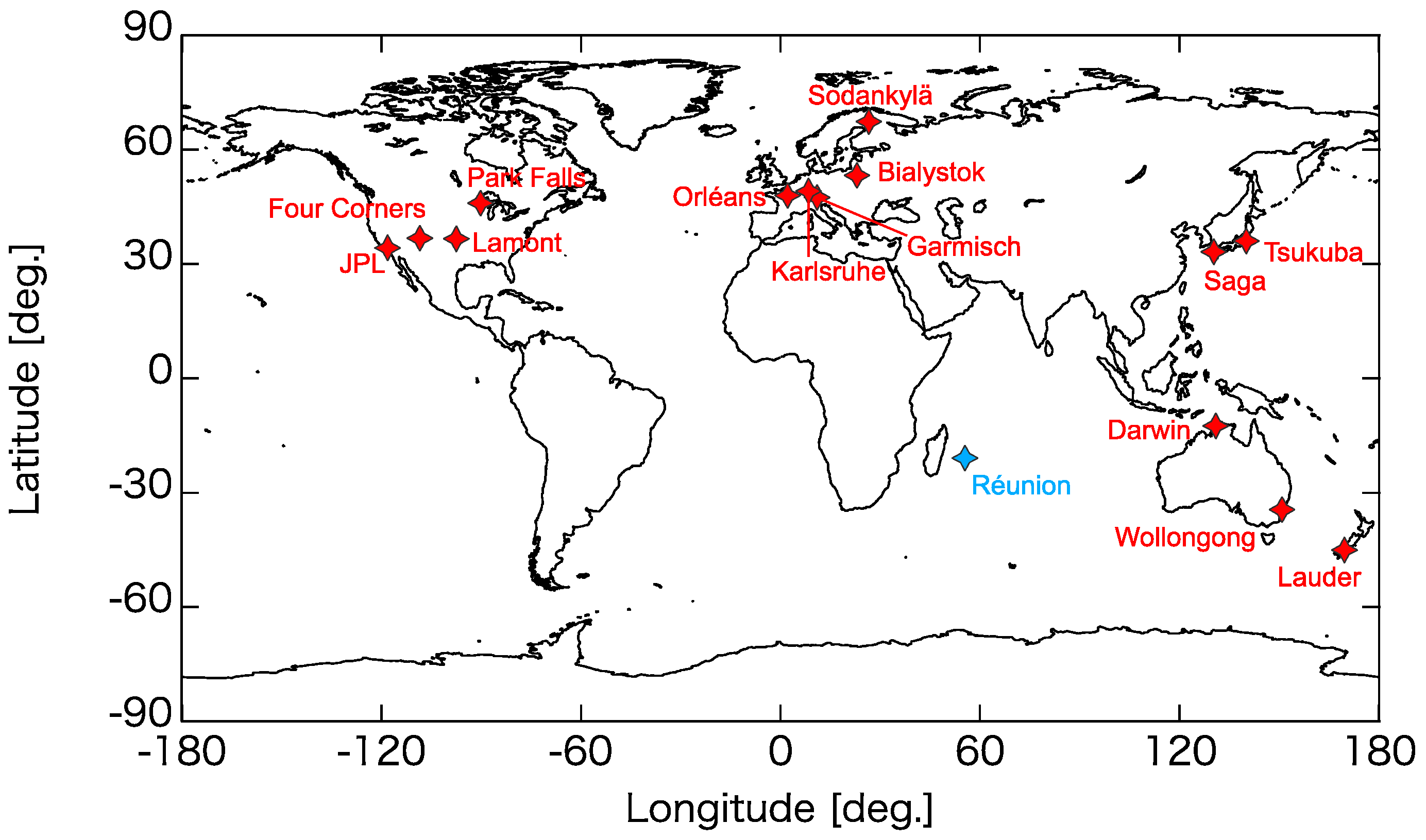
2.2. Total Carbon Column Observing Network (TCCON) XH₂O

Measurements of column abundances of atmospheric greenhouse gases with a ground-based high-resolution FTS recording direct sunlight spectra have been performed at more than 20 sites in the world [19], and the network is called TCCON. The TCCON only measures during clear-sky conditions. Currently, XCO₂ and XCH₄ from TCCON are used for validating the equivalent TANSO-FTS SWIR products (e.g., [33,40]). Additionally, XCO, XN₂O, XH₂O, XHDO, and XHF are retrieved from the ground-based FTS spectra. In the present study, the XH₂O product was compared with the TANSO-FTS TIR and SWIR products. The XH₂O value was calculated by taking the ratio of the IWV and dry-air column abundances. The dry-air column was obtained from the O₂ column retrieved from the same spectra as IWV (i.e., dry-air column = O₂ column/0.2095, where the constant is the assumed dry-air mole fraction of O₂). The retrieval processing was performed by scaling an a priori profile to produce a synthetic spectrum that best fits to the measured spectrum. The a priori profiles of H₂O and temperature profile were taken from the National Centers for Environmental Prediction (NCEP) reanalysis data. The TCCON XH₂O data have been calibrated with in situ data from aircraft observations and radiosonde observations above each site, and the accuracy (1σ) of the TCCON XH₂O data was estimated to be 5% [41].

For the TANSO-FTS data to be compared with the TCCON data, we selected the TANSO-FTS data that were within circles with radii of 50, 75, 100, 150 or 200 km from the TCCON site. For each case, the TCCON data were averaged within ±10 min of the GOSAT overpass, and the averaged values were compared with the TANSO-FTS data. We selected the TCCON sites with the solar absorption spectra acquired for more than two years within the period from April 2009 to May 2014. The TCCON sites with more than ten matching pairs against the SWIR product, in the case of the spatial coincidence criterion of 100 km, were employed. Application of these criteria resulted in the omission of the Eureka, Ny-Ålesund, Bremen, Izaña, and Réunion sites from intercomparison. However, the Réunion site was used only for comparison with the TANSO-FTS TIR data above ocean. Figure 1 shows the locations of a total of 15 TCCON sites used in the present study. Each TCCON site adopts almost identical instrumentation and data acquisition procedures. In addition, a common software package is used for data processing and analysis. The XH₂O data derived using the GGG2014 software package were available for Sodankylä [42], Białystok [43], Karlsruhe [44], Orléans [45], Garmisch [46], Park Falls [47], Lamont [48], Tsukuba [49], JPL [50], Saga [51], Darwin [52], Réunion [53], Wollongong [54] and Lauder [55,56], whereas for the Four Corners site, we used the GGG2012 XH₂O data.

3. Methods

The TANSO-FTS has only one footprint that is scanned every 4 s, and the neighboring measurements of the TANSO-FTS are usually more than 200 km apart. Even around the TCCON sites, few near-coincident measurements are performed. Therefore, we cannot evaluate the precision of TANSO-FTS data from the successive measurements. In the cases of CO₂ and CH₄, which have lower spatial variability compared with H₂O, the standard deviation of the mean difference between the TANSO-FTS and TCCON data can be regarded as precision (e.g., [40,57]). However, in the case of H₂O with high spatial variability, the standard deviation includes the effects of the spatial (and temporal) variability, as well as the precisions. Therefore, we determine the precisions and spatial variability by an intercomparison between three datasets after the corrections described in Section 3.1 and Section 3.2.

3.1. Correction of Difference in Elevation

The difference in XH₂O values resulting from the difference in elevations between TANSO-FTS IFOV and TCCON site required correction. We adjusted the IWV and dry-air column in the TANSO-FTS data individually to those at the TCCON site elevation. First, the IWV in the TANSO-FTS TIR or SWIR data $C_{\mathrm{IWV}}$ were corrected using Equation (1):

$$C_{\mathrm{IWV}}^{\prime }=C_{\mathrm{IWV}}(1+\Gamma \cdot \Delta h)$$

(1)

where Δh is the altitude difference between the TANSO-FTS IFOV and TCCON sites (TANSO-FTS minus TCCON) and Г is the rate of change of the IWV with respect to altitude change, which was derived using the radiosonde data according to a method described in Buehler et al. [5]. This group pointed out that the Г value is dependent on season and location, and, therefore, we derived the monthly mean Г values for the respective TCCON sites using radiosonde data during the period from 2009 to 2014. The radiosonde data were obtained from the Integrated Global Radiosonde Archive [58]. The radiosonde launch sites corresponding to each TCCON site are listed in Table S1 in the supplementary material. The derived Г values are given in percent per 100 m. They are summarized in Table S2 in the supplementary material and range from 3.2 to 4.8.

Second, the total air columns in the TANSO-FTS TIR or SWIR data $C_{\mathrm{AIR}}$, which were derived from the GPV data, were corrected using the following equation:

$$C_{\mathrm{AIR}}^{\prime }=C_{\mathrm{AIR}}\exp \left(\Delta h/h_{\mathrm{s}}\right)$$

(2)

where $h_{\mathrm{s}}$ is the scale height. The scale height can be expressed by the following equation [59]:

$$h_{\mathrm{s}}=R{T}_{\mathrm{g}}/Mg$$

(3)

where R is the mole gas constant, M is the average molecular weight of wet air (28.97 g∙mol⁻¹ [59]), g is the gravitational acceleration, and $T_{\mathrm{g}}$ is the atmospheric temperature taken at each TCCON site that was included in the TCCON data. The corrected dry-air columns in the TANSO-FTS TIR or SWIR data were derived by subtracting $C_{\mathrm{IWV}}^{\prime }$ from $C_{\mathrm{AIR}}^{\prime }$. We note that the TANSO-FTS data were adjusted for both negative and positive altitude differences.

Some radiosonde sites are outside the largest spatial coincidence criterion of 200 km radius around the TCCON site. We evaluated the impact of the large distance by comparing altitude correction results of TANSO-FTS SWIR XH₂O data around the Saga TCCON site using radiosondes at Fukuoka and Kagoshima, which are 39 km and 182 km away from Saga, respectively. Figure S1 in the supplementary material shows the Г values for relatively close radiosonde sites; the distances are 69 km for Altenstadt and München, 154 km for Akita and Misawa, and 218 km for Fukuoka and Kagoshima. The mean difference between the TANSO-FTS SWIR XH₂O data corrected based on the different radiosonde data (Kagoshima minus Fukuoka) was −0.13% (−2.0 ppm) with a standard deviation of 0.39% (6.3 ppm).

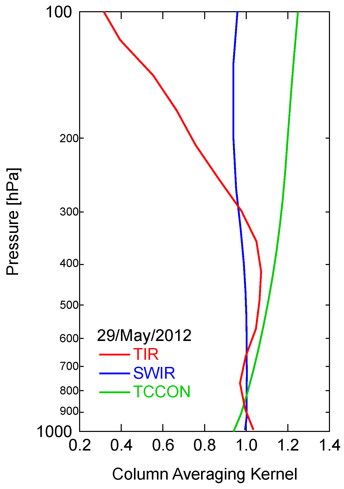
3.2. Correction of the Difference in a Priori H₂O Profile

In order to accurately compare physical quantities obtained from the two kinds of remote sensing instruments, it is necessary to consider the effects of differences in a priori profile and vertical resolution (i.e., column averaging kernel). The latter is considered in the next section, and the method for correcting the effect of the former is described here. The TCCON a priori profile of H₂O was taken from the NCEP reanalysis data, while both the TANSO-FTS TIR and SWIR retrieval algorithms used the GPV data. To conform to a common a priori profile, the TCCON XH₂O data ${\widehat{c}}_{\mathrm{TCCON}}$ were adjusted to the TANSO-FTS a priori profile according to Rodgers and Connor [60]:

$${\widehat{c}}_{\mathrm{TCCON}}^{\prime }={\widehat{c}}_{\mathrm{TCCON}}+{\displaystyle \sum _j{h}_j}{(a_{\mathrm{TCCON}}-u)}_j{(x_{\mathrm{TCCON}}^a-x_{\mathrm{TANSO}}^a)}_j$$

(4)

where $a_{\mathrm{TCCON}}$ is the column averaging kernel for TCCON, u is the unit vector, h is the pressure-weighting function of the dry-air partial column, and $x_{\mathrm{TCCON}}^a$ and $a_{\mathrm{TCCON}}$ are the a priori profiles of H₂O for TCCON and TANSO-FTS, respectively. The TANSO-FTS a priori profile was re-gridded by linearly interpolating it to the TCCON vertical grid. Thus, we compared the TCCON XH₂O data adjusted to the TANSO-FTS a priori profile of H₂O (${\widehat{c}}_{\mathrm{TCCON}}^{\prime }$) with the TANSO-FTS TIR or SWIR XH₂O data.

Aside from the a priori correction for the TCCON XH₂O data, we evaluated a priori profile contribution on the TANSO-FTS XH₂O data based on a ratio of ${\displaystyle {\sum }_j{h}_j{(u-a_{\mathrm{TANSO}})}_j{x}_{\mathrm{TANSO}j}^a}$ and retrieved XH₂O. The a priori contributions on the TANSO-FTS TIR and SWIR XH₂O data, which were calculated as the mean absolute value of those ratios around the TCCON sites, were 4.5% and 0.21%, respectively.

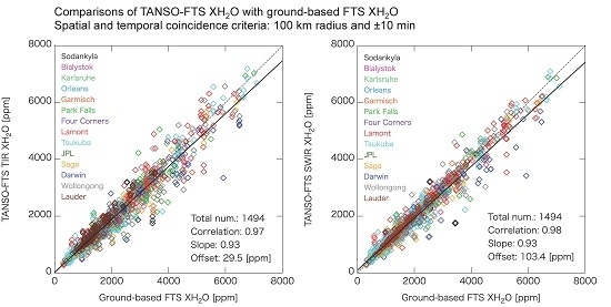
3.3. Intercomparison between Three Datasets

In comparing the XH₂O data from two instruments, a mean difference (systematic bias) with a standard deviation (dispersion) would exist. The TCCON XH₂O data were calibrated as described in Section 2.2. Thus, the TCCON data was regarded as a reference. The mean difference against the TCCON data was evaluated as the bias of the TANSO-FTS data. For the comparison between the TANSO-FTS TIR and TANSO-FTS SWIR XH₂O (${\widehat{c}}_{\mathrm{TIR}}$ and ${\widehat{c}}_{\mathrm{SWIR}}$), a bias was calculated from the individual difference defined as:

$$\Delta =\frac{({\widehat{c}}_{\mathrm{TIR}}-{\widehat{c}}_{\mathrm{SWIR}})}{({\widehat{c}}_{\mathrm{TIR}}+{\widehat{c}}_{\mathrm{SWIR}})/2}$$

(5)

In comparing the TANSO-FTS (TIR and SWIR) and TCCON data, the square of the standard deviation (i.e., variance) was expressed by Equation (6) for TIR-TCCON pair and Equation (7) for SWIR-TCCON pair:

$${\sigma }_{\mathrm{TIR}-\mathrm{TCCON}}^2={\sigma }_{\mathrm{TIR}}^2+{\sigma }_{\mathrm{TCCON}}^2+{\sigma }_{\mathrm{R}(\mathrm{TIR}-\mathrm{TCCON})}^2+{\sigma }_{\mathrm{S}}^2$$

(6)

$${\sigma }_{\mathrm{SWIR}-\mathrm{TCCON}}^2={\sigma }_{\mathrm{SWIR}}^2+{\sigma }_{\mathrm{TCCON}}^2+{\sigma }_{\mathrm{R}(\mathrm{SWIR}-\mathrm{TCCON})}^2+{\sigma }_{\mathrm{S}}^2$$

(7)

where ${\sigma }_{\mathrm{TIR}}^2$, ${\sigma }_{\mathrm{SWIR}}^2$, and ${\sigma }_{\mathrm{TCCON}}^2$ are the variances of the TIR, SWIR, and TCCON XH₂O data, respectively. ${\sigma }_{\mathrm{R}(\mathrm{TIR}-\mathrm{TCCON})}^2$ and ${\sigma }_{\mathrm{R}(\mathrm{SWIR}-\mathrm{TCCON})}^2$ are the variances resulting from the difference in the vertical resolutions of the TANSO-FTS (TIR and SWIR) and TCCON XH₂O data, and ${\sigma }_{\mathrm{S}}^2$ is the variance representative of spatial variability of XH₂O. The ${\sigma }_{\mathrm{TIR}-\mathrm{TCCON}}$ and ${\sigma }_{\mathrm{SWIR}-\mathrm{TCCON}}$ values for each TCCON site were obtained by calculating the standard deviation of the differences between the TANSO-FTS XH₂O bias-corrected with respect to the TCCON XH₂O data and the TCCON data. For comparing the TANSO-FTS TIR and SWIR data, we did not need to take into account ${\sigma }_{\mathrm{S}}^2$ because TANSO-FTS measures the TIR and SWIR spectra simultaneously at the same IFOV. The variance between the TANSO-FTS TIR and SWIR data is, therefore, given by

$${\sigma }_{\mathrm{TIR}-\mathrm{SWIR}}^2={\sigma }_{\mathrm{TIR}}^2+{\sigma }_{\mathrm{SWIR}}^2+{\sigma }_{\mathrm{R}(\mathrm{TIR}-\mathrm{SWIR})}^2$$

(8)

where ${\sigma }_{\mathrm{R}(\mathrm{TIR}-\mathrm{SWIR})}^2$ is the variance resulting from the difference in the vertical resolutions of the TANSO-FTS TIR and SWIR XH₂O data. We must note that, for Equation (8) to be true, it is crucial that the TANSO-FTS TIR XH₂O data are independent of the TANSO-FTS SWIR data. This is discussed in Appendix A.

The variance resulting from the difference in the vertical resolutions of two instruments 1 and 2 can be calculated from the following equation [40,60]:

$${\sigma }_{\mathrm{R}(1-2)}^2={\displaystyle \sum _k{\displaystyle \sum _j{h}_j(}{a}_1-a_2{)}_j{(S_{\mathrm{c}})}_{jk}{h}_k{(a_1-a_2)}_k}$$

(9)

where $a_1$ and $a_2$ are the column averaging kernel for instruments 1 and 2, respectively, and $S_{\mathrm{c}}$ is the ensemble covariance matrix of H₂O. However, since it is difficult to evaluate the $S_{\mathrm{c}}$ values for each site, we evaluated the difference in XH₂O values resulting from the difference in column averaging kernels, according to Rodgers and Connor [60]:

$$\delta ={\displaystyle \sum _j{h}_j{(a_1-a_2)}_j{(x-x_{\mathrm{TANSO}}^a)}_j}$$

(10)

where x is the true H₂O profile, corresponding here to radiosonde H₂O profile. We approximate ${\sigma }_{\mathrm{R}(1-2)}$ by the standard deviation of δ, calculated for a set of true values, x. The δ values were evaluated using H₂O profiles obtained from radiosonde measurements during the period from 2009 to 2014, which were performed near each TCCON site listed in Table S1. The respective profiles were linearly interpolated or extrapolated to the TCCON site’s altitude. It should be noted that the variability of the δ values could be an overestimate because the radiosonde data have biases of their own and the spatio-temporal discrepancies of radiosonde and TANSO-FTS/TCCON measurements might introduce significant variability. An example of column averaging kernels of TANSO-FTS TIR, TANSO-FTS SWIR, and ground-based FTS measurements at Saga, Japan is shown in Figure 2. The ${\sigma }_{\mathrm{R}(\mathrm{TIR}-\mathrm{TCCON})}$, ${\sigma }_{\mathrm{R}(\mathrm{SWIR}-\mathrm{TCCON})}$ and ${\sigma }_{\mathrm{R}(\mathrm{TIR}-\mathrm{SWIR})}$ values obtained from the TANSO-FTS measurements within 100 km distance from the TCCON site are summarized in

Table 1. Standard deviations of the differences in the XH₂O values resulting from the difference in the vertical resolutions of the two instruments (${\sigma }_{\mathrm{R}}$) and the difference of mean altitude of the TANSO-FTS footprint to the TCCON site’s altitude.

TCCON Sites	${\mathit{\sigma }}_{\mathbf{R}(\mathbf{TIR}-\mathbf{TCCON})}$ (%)	${\mathit{\sigma }}_{\mathbf{R}(\mathbf{SWIR}-\mathbf{TCCON})}$ (%)	${\mathit{\sigma }}_{\mathbf{R}(\mathbf{TIR}-\mathbf{SWIR})}$ (%)	Mean ∆h (m)
Sodankylä	3.2	0.88	1.5	80
Białystok	4.4	0.93	1.8	−17
Karlsruhe	2.2	0.77	1.8	190
Orléans	2.3	0.92	1.9	−13
Garmisch	2.2	0.57	1.0	−48
Park Falls	3.8	1.7	2.1	37
Four Corners	3.2	2.5	2.5	311
Lamont	2.0	0.83	2.1	−6
Tsukuba	2.3	0.88	2.4	29
JPL	4.2	1.7	3.0	−97
Saga	2.6	0.95	3.5	111
Darwin	2.1	1.1	3.1	4
Wollongong	2.8	1.6	2.7	434
Lauder	3.7	1.3	4.0	58
All sites	2.8	1.2	2.5	85

. Table 1 also lists the difference between mean altitude of the TANSO-FTS footprint and the TCCON site’s altitude. The mean altitude of the TANSO-FTS footprint around a TCCON site was determined by calculating an arithmetic mean of the average altitudes within the respective TANSO-FTS footprints around the TCCON site. We found that the amplitude and site dependence of ${\sigma }_{\mathrm{R}}$ values for the SWIR-TCCON pair were smaller than those for the TIR-TCCON and TIR-SWIR pairs. In addition, the ${\sigma }_{\mathrm{R}}$ values were independent of the difference between the mean altitude of the TANSO-FTS footprint and the TCCON site’s altitude.

The relative variability of TCCON XH₂O, ${\sigma }_{\mathrm{TCCON}}$, was estimated from the mean value $m_{\mathrm{TCCON}}$ and its standard deviation $s_{\mathrm{TCCON}}$ during ±10 min of the GOSAT overpass time, as $s_{\mathrm{TCCON}}/m_{\mathrm{TCCON}}$. Since the ground-based FTS acquires one spectrum per approximately 1 min, the ${\sigma }_{\mathrm{TCCON}}$ value was calculated from 20 TCCON data at a maximum. The average ${\sigma }_{\mathrm{TIR}-\mathrm{TCCON}}$, ${\sigma }_{\mathrm{SWIR}-\mathrm{TCCON}}$, ${\sigma }_{\mathrm{TIR}-\mathrm{SWIR}}$, ${\sigma }_{\mathrm{TCCON}}$ and ${\sigma }_{\mathrm{R}}$ values for all TCCON sites were calculated as an ensemble of all data from each site. Finally, the unknown variables ${\sigma }_{\mathrm{TIR}}$, ${\sigma }_{\mathrm{SWIR}}$ and ${\sigma }_{\mathrm{S}}$ were determined using Equations (6) to (8).

4. Results

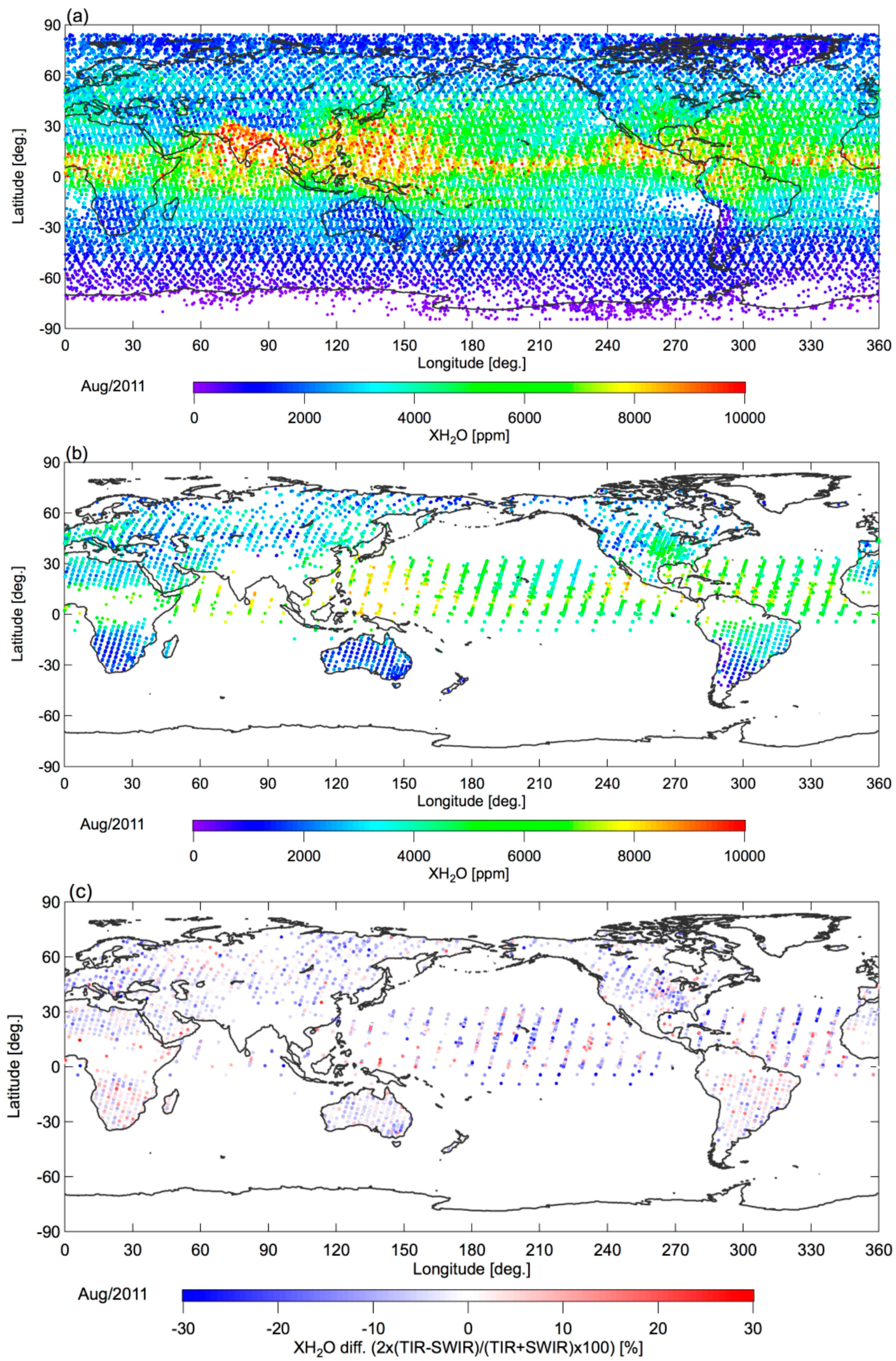
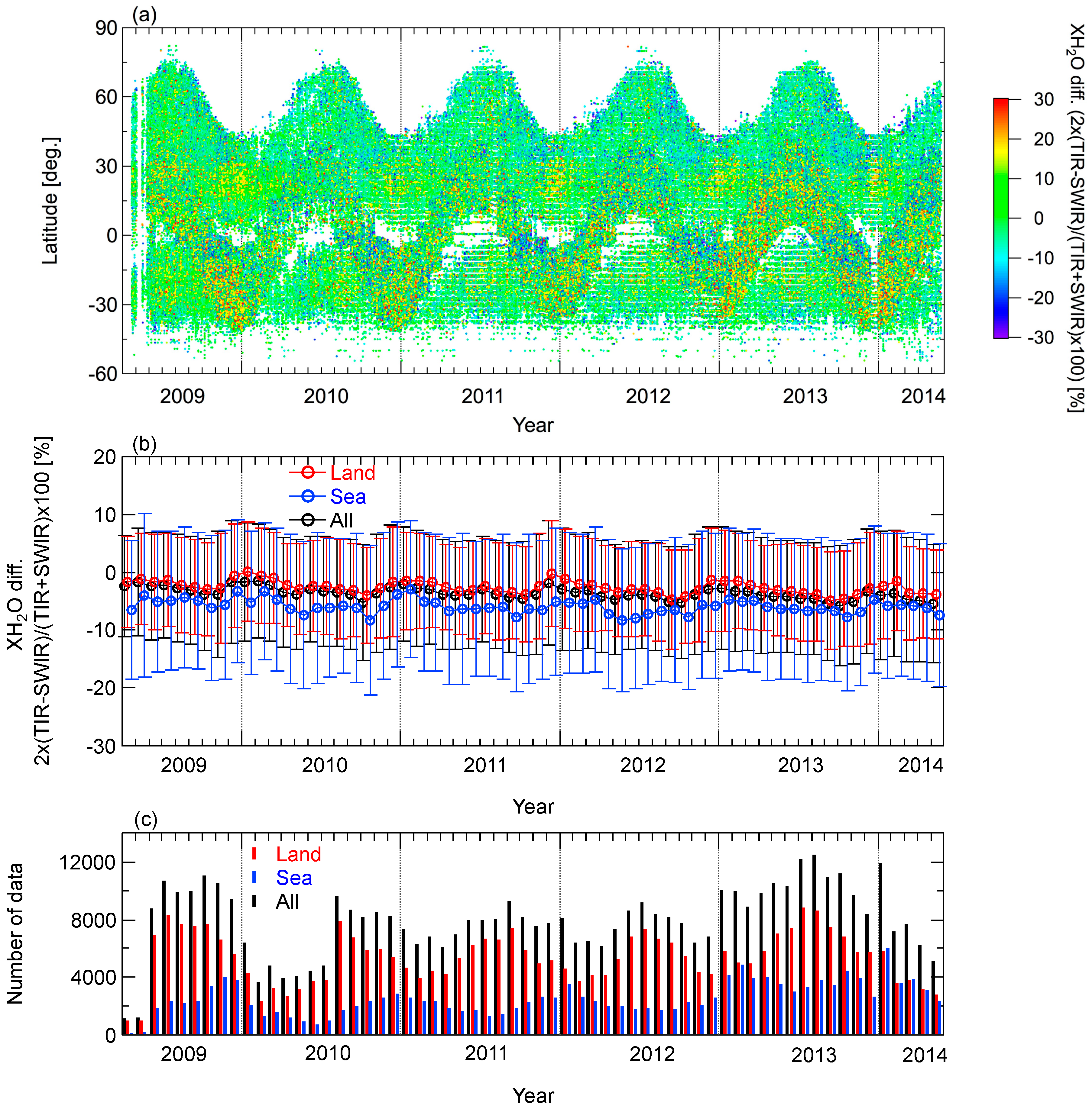
4.1. Comparisons between Global TANSO-FTS TIR and SWIR XH₂O

Figure 3a,b shows global distributions of the TANSO-FTS TIR and TANSO-FTS SWIR XH₂O data in August 2011, respectively. Figure 3c shows the differences between the TANSO-FTS TIR and SWIR XH₂O data for exactly the same scene. Figure 4a indicates time-latitude cross-sections of the differences between the TANSO-FTS TIR and SWIR XH₂O data during the period from April 2009 to May 2014. The latitudinal range for the matching between the TANSO-FTS TIR and SWIR data changes seasonally, especially in the Northern Hemisphere, because the TANSO-FTS SWIR retrievals are limited to the solar zenith angle (SZA) of less than 70°. The mean difference for all data is −3.7% with a standard deviation of 10.0%. The monthly mean differences and their standard deviations (1σ) are shown individually for land, ocean, and all (land + ocean) scenes in Figure 4b, and the amounts of data employed for comparisons are shown in Figure 4c. The mean differences above land and ocean are −2.7% ± 8.4% and −5.9% ± 12.5%, respectively. The standard deviation for the ocean scenes was larger than that for the land scenes. The ocean and land differences are further investigated in Section 4.2.2, and we used the TANSO-FTS XH₂O data only above land in the following intercomparison.

Figure 5 shows the differences between the TANSO-FTS TIR and SWIR XH₂O data above land with respect to SZA. The absolute values of the mean bias became larger with increasing SZA, and this may be attributed to an error in the air-mass factor in radiative transfer in the SWIR region. The standard deviation of the difference also became larger with increasing SZA (i.e., 6.9%, 7.1%, 7.6%, 8.1%, 8.7%, 9.4% and 9.9% for the increasing SZA bin), and this likely resulted from a mismatch volume of atmosphere between TANSO-FTS TIR and SWIR observations, whose magnitude varied with SZA as shown in Figure 6. The radiation in the TIR and SWIR regions observed with the TANSO-FTS does not pass through the exact same volume of atmosphere, because the latter is the backscattered solar radiation that passes through atmosphere twice (i.e., solar to ground surface and ground surface to satellite). Since it is difficult to correct or take into account the effect of the mismatch volume, we will estimate the errors in ${\sigma }_{\mathrm{TIR}}$, ${\sigma }_{\mathrm{SWIR}}$ and ${\sigma }_{\mathrm{S}}$ caused by ignoring the mismatch volume in Section 5.1.

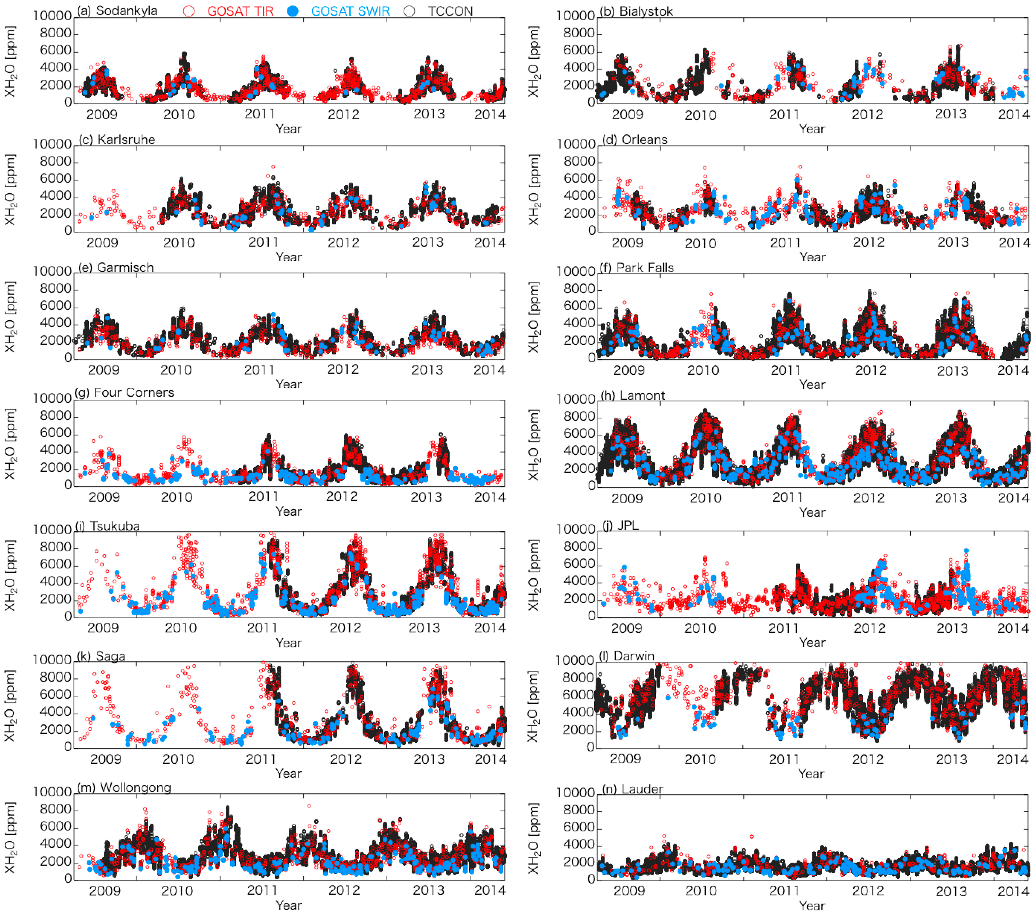
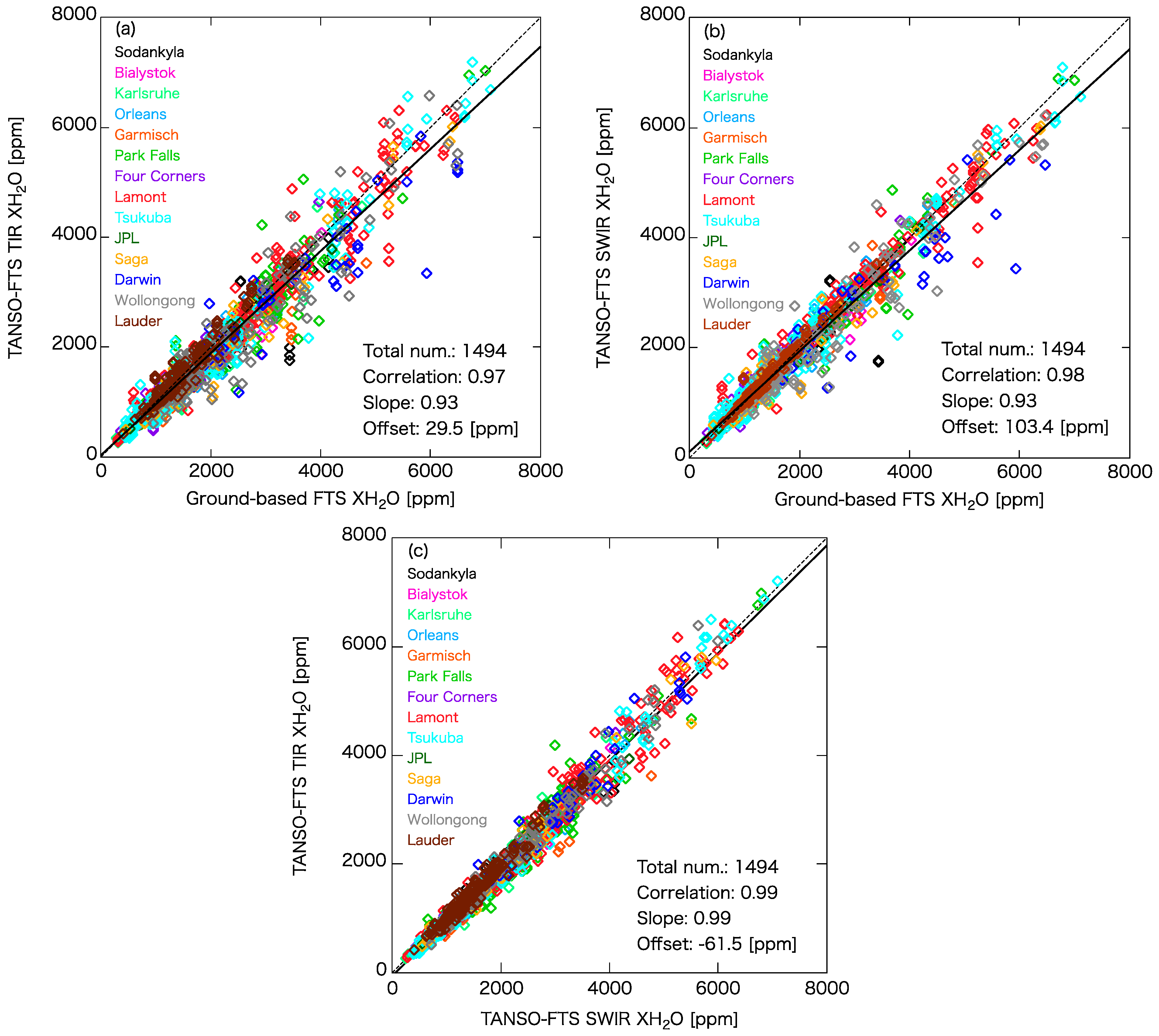
4.2. Intercomparisons of XH₂O around TCCON Sites

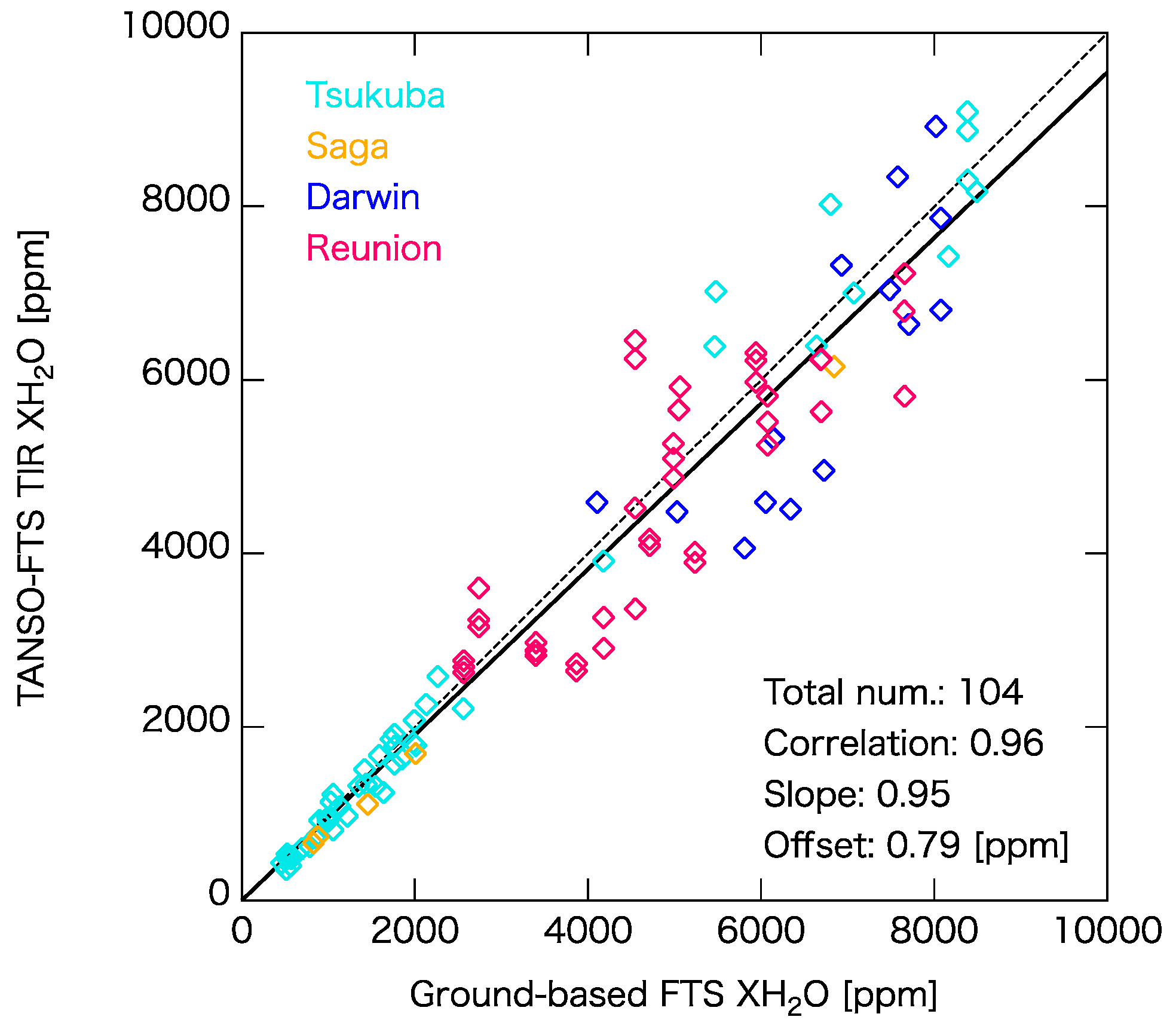
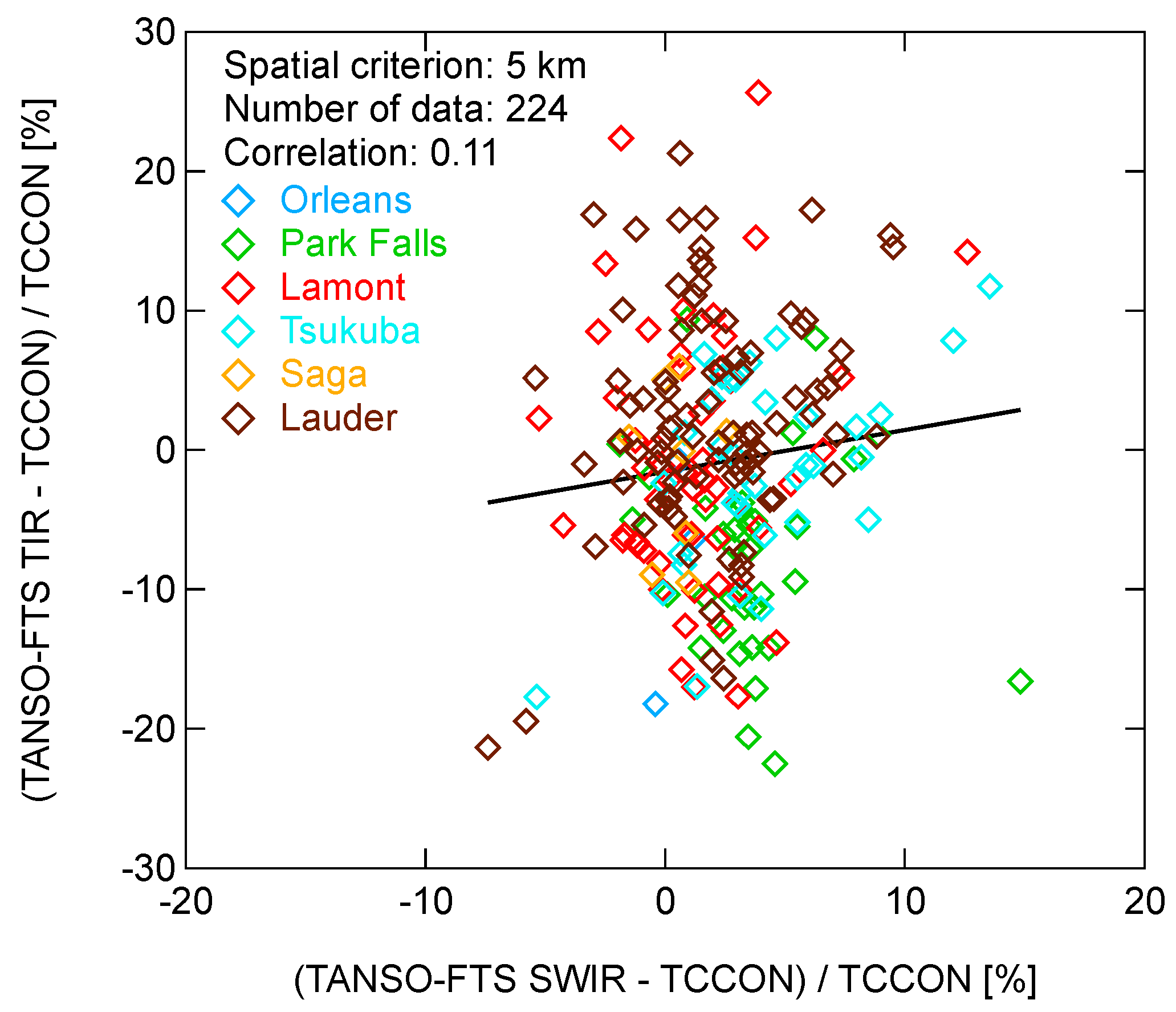
4.2.1. Comparisons of TANSO-FTS XH₂O above Land with TCCON XH₂O

We made an intercomparison between the TANSO-FTS XH₂O data above land and the TCCON XH₂O data. We first describe the results using the spatial coincidence criterion of 100 km, and then discuss them using different spatial coincidence criteria in Section 4.3. Figure 7a–n shows the time series of XH₂O at the respective TCCON sites. Note that the TANSO-FTS TIR data in both daytime and nighttime are shown. The TANSO-FTS TIR and SWIR measurements could observe seasonal variations of XH₂O similar to the TCCON measurements. The TCCON measurements at the six sites (Karlsruhe, Orleans, Four Corners, Tsukuba, JPL and Saga) were started after the beginning of the TANSO-FTS observation. Multiple gaps are present in the TCCON data due to instrumental trouble, rainy season, and high SZA condition. Similarly, the number of TANSO-FTS SWIR data in the rainy season and the high SZA condition is relatively low. In addition, few TANSO-FTS SWIR data are available in cases where the XH₂O data for TCCON and TANSO-FTS TIR exceed 7000 ppm. If water vapor amount is large, then spectral residual (difference between observed and calculated spectra) due to inaccuracies in spectroscopic parameters of H₂O also becomes large. The TANSO-FTS SWIR data with the large residual (i.e., large XH₂O) are screened out in post-processing [38]. The TANSO-FTS TIR data were steadily acquired for each site during the considered period.

In order to accurately determine the spatial variability, ${\sigma }_{\mathrm{S}}$, the mutually coincident TANSO-FTS TIR, TANSO-FTS SWIR, and TCCON XH₂O data were intercompared. Figure 8a shows a correlation plot between the TANSO-FTS TIR and TCCON values. The TANSO-FTS data were corrected to take into account the difference in elevation between the TANSO-FTS IFOV and the TCCON site, as described in Section 3.1. The TCCON data were adjusted to the TANSO-FTS a priori profile of H₂O, as described in Section 3.2, and the adjusted values were averaged within ±10 min of the GOSAT overpass time. The mean difference between the adjusted and the raw TCCON XH₂O data (adjusted minus raw data) is −1.4% (−20.3 ppm) with a standard deviation of 2.0% (35.4 ppm).

Table 2. Mean biases (Δ) and their standard deviations (σ) of the differences between the XH₂O data. The amount of data used for the intercomparison and the mean TCCON XH₂O values are also listed.

TCCON Sites (Alt. (m))	TIR-TCCON		SWIR-TCCON		TIR-SWIR		Mean TCCON XH2O (ppm)	N
	Δ (%)	σ (%)	Δ (%)	σ (%)	Δ (%)	σ (%)
Sodankylä (188)	−6.6	17.0	−2.7	16.7	−4.8	8.1	2176.5	44
Białystok (180)	−11.5	12.2	−4.3	9.8	−8.1	8.1	2282.2	18
Karlsruhe (116)	−10.0	16.7	−3.4	11.6	−7.5	12.9	2166.2	30
Orléans (130)	−8.4	12.4	−1.1	9.3	−8.1	8.3	2035.3	62
Garmisch (740)	−16.2	17.3	−4.0	11.7	−15.1	10.4	2331.0	27
Park Falls (440)	−6.2	15.1	0.21	11.6	−6.5	10.9	2301.0	166
Four Corners (1643)	−2.0	15.7	6.0	13.9	−3.7	6.1	1095.0	98
Lamont (320)	−1.4	14.3	2.2	13.8	−3.7	8.7	2509.5	280
Tsukuba (30)	−4.0	15.5	2.5	15.0	−6.8	7.6	1564.0	341
JPL (390)	−3.0	5.6	−5.2	3.8	1.2	4.8	2485.0	13
Saga (8)	−8.4	16.0	−2.4	15.2	−5.8	8.5	2070.1	66
Darwin (30)	−10.6	17.9	−9.1	16.3	−2.2	7.7	3408.4	52
Wollongong (30)	−9.1	17.3	−3.9	15.7	−5.1	7.9	2554.2	137
Lauder (370)	3.5	10.3	3.4	7.3	−0.54	7.5	1571.6	160
All sites	−4.4	15.0	0.63	13.4	−5.0	8.8	2050.7	1494

(second and third columns) lists the mean biases and their standard deviations between the TANSO-FTS TIR and TCCON XH₂O data for each TCCON site. For the 14 TCCON sites, the total bias of the TANSO-FTS TIR data to the TCCON data was −4.4% with a standard deviation of 15.0%, and the correlation coefficient was 0.97. The ${\sigma }_{\mathrm{TIR}-\mathrm{TCCON}}$ value in Equation (6) corresponds to this standard deviation.

Figure 8b shows a correlation plot between the TANSO-FTS SWIR and TCCON XH₂O data. The coincidence criteria and correction methods are similar to those used in the comparison between TANSO-FTS TIR and TCCON. The fourth and fifth columns in Table 2 list the mean biases and their standard deviations between the TANSO-FTS SWIR and TCCON XH₂O data for each TCCON site. The total bias was 0.63% with a standard deviation (${\sigma }_{\mathrm{SWIR}-\mathrm{TCCON}}$) of 13.4%, and the correlation coefficient was 0.98. A Student’s t-test indicates that, as a whole, there is no statistically significant bias between the TANSO-FTS SWIR and TCCON XH₂O at the 95% level of confidence. However, the ranges between the maximum and minimum of the bias across the TCCON sites are more than 15% for both TIR and SWIR. The differences at any site are more likely attributed not to instrumental but to geophysical factors, given that all the TCCON sites adopt almost identical observational setups and identical data processing methods, as described in Section 2.2.

Figure 8c shows a correlation plot between the TANSO-FTS TIR and SWIR XH₂O data within 100 km distance from the TCCON sites, and Table 2 (fourth column) lists the standard deviations of the differences between the TANSO-FTS TIR and SWIR data for the respective sites. The total bias of the TANSO-FTS TIR data to the TANSO-FTS SWIR data was −5.0% with a standard deviation of 8.8%, and the correlation coefficient was 0.99. This small standard deviation, smaller than those derived from the comparisons to the TCCON data, is attributed to the same IFOV (i.e., there is no ${\sigma }_{\mathrm{S}}$ term on the right-hand side of Equation (8)). The standard deviation was almost equal to that derived from the comparison of global TANSO-FTS TIR and SWIR land scenes (Section 4.1), whereas the mean bias became more negative by ~3 percentage points. In addition, the standard deviations for the satellite product differences over the respective TCCON sites ranged from 4.8% to 12.9%, whereas the mean biases ranged from −15.1% to 1.2%. Thus, it was determined that site (space) dependence of mean bias is larger than that of standard deviation.

To investigate the effects of the differences in column averaging kernel between TANSO-FTS and TCCON on the biases in the TANSO-FTS XH₂O data, the TCCON data were smoothed by the TANSO-FTS column averaging kernel to simulate what the TANSO-FTS would observe, provided that the TCCON data were true [40,60]. The mean difference between the TCCON XH₂O data smoothed by the TANSO-FTS TIR column averaging kernel and the raw TCCON XH₂O data (smoothed minus raw data) was −0.10% with a standard deviation of 1.5%. The mean difference in the case of the TANSO-FTS SWIR column averaging kernel was found to be an order of magnitude less than the mean difference for TIR. These results demonstrate that the effects of the column averaging kernel on the biases in the TANSO-FTS data are negligibly small.

4.2.2. Comparisons of TANSO-FTS TIR XH₂O above Ocean with TCCON XH₂O

We found that the standard deviation for the ocean scenes was larger than that for the land scenes from the comparisons between global TANSO-FTS TIR and SWIR XH₂O data in Section 4.1. To investigate whether the larger standard deviation above ocean results from the TANSO-FTS TIR or TANSO-FTS SWIR XH₂O data, the TANSO-FTS XH₂O data only above ocean were compared with the TCCON data. The TCCON sites, from which the TANSO-FTS TIR data within a radius of 100 km exist, were selected, namely the Tsukuba, Saga, Darwin, and Réunion (20.90°S, 55.49°E) sites. Note that the Izaña site (28.30°N, 16.48°W) was not used due to the large difference between elevation at the ground-based FTS site (2367 m) and average elevation within the TANSO-FTS IFOV (sea level). The TANSO-FTS SWIR XH₂O data could not sufficiently match up with the TCCON data, because the TANSO-FTS SWIR data were mainly limited to the sunglint scenes. Figure 9 shows the correlation plot between the TANSO-FTS TIR and TCCON XH₂O data. The mean difference between the TANSO-FTS TIR and TCCON XH₂O was −6.6% ± 15.7%. The standard deviation for the ocean scene was comparable to that of the land scene (15.0%). The TANSO-FTS TIR XH₂O retrieval algorithm dealt equally with land and ocean scenes, while the TANSO-FTS SWIR XH₂O retrieval algorithm derived different parameters for land and ocean scenes (i.e., surface albedo at discrete wavenumber grids for land and surface wind speed and radiance-offset values for the ocean). The handling of the ocean scene in the TANSO-FTS SWIR retrieval algorithm may have caused the larger difference between the TANSO-FTS TIR and SWIR XH₂O above ocean. Validation of the TANSO-FTS SWIR XH₂O data above ocean is beyond the scope of the current investigation and will be the subject of a future study.

4.3. Evaluations of TANSO-FTS XH₂O Precisions and Spatial XH₂O Variability

The terms on the left side of Equations (6)–(8) are derived in Section 4.2.1. The third terms on the right-hand side of Equations (6)–(8) are approximated in Section 3.3 by Equation (10), and collated in Table 1. The variability of the TCCON XH₂O data within ±10 min of the GOSAT overpass (i.e., precision of TCCON data, ${\sigma }_{\mathrm{TCCON}}$) is listed in

Table 3. Standard deviations of the TCCON XH₂O data within ±10, ±20, ±60 and ±120 min of the GOSAT overpass time.

TCCON Sites	${\mathit{\sigma }}_{\mathbf{TCCON}}$ (%)
	±10 (min)	±20 (min)	±60 (min)	±120 (min)
Sodankylä	1.2	1.7	2.4	3.7
Białystok	1.1	1.3	2.7	3.9
Karlsruhe	1.2	1.6	2.6	3.3
Orléans	1.4	1.9	2.5	3.5
Garmisch	1.3	1.7	3.6	5.4
Park Falls	2.1	2.5	4.1	6.2
Four Corners	1.7	2.3	3.8	5.0
Lamont	1.6	2.3	3.6	5.1
Tsukuba	2.0	2.8	4.6	6.7
JPL	1.0	1.4	2.6	4.0
Saga	1.9	2.4	3.8	5.2
Darwin	1.9	2.4	3.9	4.7
Wollongong	1.6	2.2	4.0	6.8
Lauder	1.7	2.3	3.5	5.0
All sites	1.8	2.4	3.8	5.5

, and the ${\sigma }_{\mathrm{TCCON}}$ value amounts to 1.8%. Finally, the unknown variables ${\sigma }_{\mathrm{TIR}}$, ${\sigma }_{\mathrm{SWIR}}$, and ${\sigma }_{\mathrm{S}}$ were solved using Equations (6)–(8), and the resulting ${\sigma }_{\mathrm{TIR}}$, ${\sigma }_{\mathrm{SWIR}}$ and ${\sigma }_{\mathrm{S}}$ values were 7.4%, 4.1% and 12.6%, respectively. We found that the spatial variability ${\sigma }_{\mathrm{S}}$ accounted for a large portion of the difference between the TANSO-FTS and the TCCON XH₂O data for the spatial coincidence criterion of 100 km. We note that although the ${\sigma }_{\mathrm{TIR}}$, ${\sigma }_{\mathrm{SWIR}}$ and ${\sigma }_{\mathrm{S}}$ values could be, in principle, determined site by site, the values averaged over all the TCCON sites were derived in the present study, because there are several sites that have a statistically insufficient amount of matching pairs. The evaluation of the differences in the ${\sigma }_{\mathrm{TIR}}$, ${\sigma }_{\mathrm{SWIR}}$ and ${\sigma }_{\mathrm{S}}$ values depending on the location and season may be possible by using other H₂O data, such as precipitable water vapor from the GPS. This will be the subject of a future study.

The results using the spatial coincidence criteria of 50, 75, 150 and 200 km are summarized in

Table B1. Standard deviations of XH₂O differences resulting from the difference in the vertical resolutions of the two instruments for the spatial coincidence criteria of 50, 75, 150, and 200 km.

TCCON Sites	${\mathit{\sigma }}_{\mathbf{R}(\mathbf{TIR}-\mathbf{TCCON})}$ (%)				${\mathit{\sigma }}_{\mathbf{R}(\mathbf{SWIR}-\mathbf{TCCON})}$ (%)				${\mathit{\sigma }}_{\mathbf{R}(\mathbf{TIR}-\mathbf{SWIR})}$ (%)
	Spatial Coincidence Criteria (km)
	50	75	150	200	50	75	150	200	50	75	150	200
Sodankylä	1.6	3.5	3.0	2.7	0.64	0.76	0.97	1.1	1.7	1.7	1.4	1.5
Białystok	4.4	4.4	4.5	4.1	0.88	0.88	0.91	1.3	1.9	1.9	1.8	1.8
Karlsruhe	2.0	2.3	2.2	2.3	0.59	0.78	0.81	0.82	1.4	1.7	2.4	2.4
Orléans	2.3	2.4	2.7	2.7	1.1	0.93	0.88	1.1	1.9	2.0	1.8	1.8
Garmisch	2.1	2.1	3.0	2.8	0.56	0.52	0.74	1.1	1.2	1.1	1.7	1.7
Park Falls	3.1	3.7	4.1	4.2	1.6	1.7	1.6	1.6	2.3	2.1	2.3	2.3
Four Corners	3.0	3.2	3.3	3.2	2.2	2.3	2.6	2.5	2.6	2.6	2.5	3.0
Lamont	2.0	2.0	2.2	2.2	0.83	0.84	0.87	0.88	2.0	2.1	2.2	2.2
Tsukuba	2.1	2.1	2.3	2.5	0.84	0.83	0.93	1.1	2.2	2.3	2.4	2.4
JPL	4.2	4.2	4.0	4.0	1.7	1.7	2.3	2.3	3.0	3.0	3.1	3.1
Saga	2.7	2.7	2.6	2.6	0.83	0.92	0.94	1.1	3.2	3.1	3.5	3.5
Darwin	1.9	1.8	2.1	2.2	NA	NA	1.8	1.7	NA	NA	2.6	2.4
Wollongong	3.0	2.7	2.8	2.8	1.6	1.5	1.4	1.4	2.6	2.7	2.7	2.8
Lauder	3.7	3.7	NA	NA	1.3	1.3	NA	NA	4.0	4.0	NA	NA
All sites	2.9	2.8	2.9	2.9	1.1	1.1	1.2	1.2	2.5	2.4	2.4	2.4

,

Table B2. Standard deviations of differences between the XH₂O data for the spatial coincidence criteria of 50, 75, 150 and 200 km.

TCCON Sites	${\mathit{\sigma }}_{\mathbf{TIR}-\mathbf{TCCON}}$ (%)				${\mathit{\sigma }}_{\mathbf{SWIR}-\mathbf{TCCON}}$ (%)				${\mathit{\sigma }}_{\mathbf{TIR}-\mathbf{SWIR}}$ (%)
	Spatial Coincidence Criteria (km)
	50	75	150	200	50	75	150	200	50	75	150	200
Sodankylä	7.7	18.1	17.8	17.9	6.0	18.4	15.7	16.2	5.6	7.8	8.7	8.8
Białystok	9.0	12.5	12.9	15.5	7.6	10.1	11.6	14.2	9.2	8.6	11.1	10.4
Karlsruhe	15.6	16.6	19.2	22.2	5.8	11.2	15.7	19.3	14.7	13.4	10.5	9.9
Orléans	9.9	11.4	14.1	20.7	5.1	7.7	12.3	18.3	8.4	8.3	8.2	9.0
Garmisch	14.9	17.8	18.4	22.9	8.3	11.2	17.7	22.1	9.6	10.5	10.5	10.3
Park Falls	11.0	11.6	16.8	20.0	5.2	7.3	14.2	17.7	10.1	10.5	10.6	10.3
Four Corners	14.0	13.7	15.3	21.1	11.7	11.4	13.7	21.3	6.7	6.3	6.3	6.3
Lamont	10.7	13.1	21.0	22.0	6.8	11.0	20.7	22.1	8.9	8.5	8.4	8.3
Tsukuba	9.5	14.3	16.6	17.6	8.8	13.4	15.8	16.4	7.7	7.6	7.6	7.9
JPL	5.6	5.6	18.7	18.7	3.6	3.8	18.0	18.0	4.8	4.8	7.4	7.4
Saga	11.6	13.0	16.2	17.4	7.7	12.3	15.4	16.3	7.7	8.0	8.5	8.2
Darwin	NA	3.4	17.6	17.3	NA	7.0	17.0	16.9	NA	5.3	7.8	7.5
Wollongong	14.0	15.1	20.5	20.5	10.4	12.3	18.7	18.6	7.4	7.1	8.6	8.7
Lauder	8.7	10.3	NA	NA	4.2	7.3	NA	NA	7.5	7.5	NA	NA
All sites	10.8	13.3	18.5	20.2	7.9	11.1	17.4	19.1	8.8	8.8	8.8	8.9

,

Table B3. The amounts of data used for the XH₂O intercomparisons for the spatial coincidence criteria of 50, 75, 150 and 200 km.

TCCON Sites	N
	Spatial Coincidence Criteria (km)
	50	75	150	200
Sodankylä	4	24	63	113
Białystok	12	15	33	62
Karlsruhe	12	27	65	98
Orléans	22	42	96	151
Garmisch	16	24	50	93
Park Falls	77	122	210	267
Four Corners	33	52	103	130
Lamont	174	234	580	694
Tsukuba	156	264	357	417
JPL	13	13	98	98
Saga	32	53	67	81
Darwin	0	3	97	112
Wollongong	70	83	251	298
Lauder	146	160	NA	NA
All sites	767	1116	2070	2614

and

Table B4. Standard deviations of the TCCON XH₂O data within ±10 min of the GOSAT overpass for the spatial coincidence criteria of 50, 75, 150, and 200 km.

TCCON Sites	${\mathit{\sigma }}_{\mathbf{TCCON}}$ (%)
	Spatial Coincidence Criteria (km)
	50	75	150	200
Sodankylä	2.0	1.5	1.2	1.1
Białystok	1.0	1.1	1.1	1.3
Karlsruhe	1.5	1.3	1.2	1.1
Orléans	1.5	1.5	1.4	1.4
Garmisch	1.1	1.2	1.3	1.4
Park Falls	2.2	2.3	2.0	2.0
Four Corners	1.9	1.9	1.7	1.9
Lamont	1.6	1.6	1.5	1.5
Tsukuba	2.1	2.1	2.0	2.0
JPL	1.0	1.0	1.1	1.1
Saga	1.9	1.9	1.9	1.9
Darwin	NA	2.0	1.7	1.7
Wollongong	1.5	1.6	1.6	1.6
Lauder	1.7	1.7	NA	NA
All sites	1.8	1.8	1.7	1.6

in Appendix B. We note that for the Darwin site, no TANSO-FTS SWIR XH₂O data were available for the spatial coincidence criterion of 50 km. Additionally, the data from the Lauder site were excluded for the spatial coincidence criteria of 150 and 200 km, because the TANSO-FTS SWIR XH₂O data within 100 km from the site account for >90% of all the data within 200 km.

Table 4. Precisions of the TANSO-FTS TIR and SWIR XH₂O data (${\sigma }_{\mathrm{TIR}}$ and ${\sigma }_{\mathrm{SWIR}}$) and spatial variability (${\sigma }_{\mathrm{S}}$) with respect to the spatial coincidence criteria.

Distance (km)	${\mathit{\sigma }}_{\mathbf{TIR}}$ (%)	${\mathit{\sigma }}_{\mathbf{SWIR}}$ (%)	${\mathit{\sigma }}_{\mathbf{S}}$ (%)
50	7.7	3.5	6.7
75	7.7	3.6	10.3
100	7.4	4.1	12.6
150	7.3	4.5	16.7
200	7.3	4.5	18.5

summarizes the resulting ${\sigma }_{\mathrm{TIR}}$, ${\sigma }_{\mathrm{SWIR}}$ and ${\sigma }_{\mathrm{S}}$ values.

Table 3 also lists the ${\sigma }_{\mathrm{TCCON}}$ values for time intervals of ±20, ±60 and ±120 min, which provide a measure of the local short-term variability of XH₂O. The ${\sigma }_{\mathrm{TCCON}}$ values increase with increasing time intervals. Assuming a typical wind speed of 7 m/s (25 km/h), a new air mass will take ~2 h to reach the center of a 50 km radius circle. Therefore, the ${\sigma }_{\mathrm{TCCON}}$ value for the ±120 min time intervals corresponds approximately to the ${\sigma }_{\mathrm{S}}$ value for the 50 km spatial coincidence criterion. Actually, the ${\sigma }_{\mathrm{TCCON}}$ value that corresponds to the ±120 min time intervals is 5.5%, and the ${\sigma }_{\mathrm{S}}$ value that corresponds to the 50 km spatial coincidence criterion is 6.7%. Given an uncertainty in the assumed wind speed and a change in the wind direction, the ${\sigma }_{\mathrm{TCCON}}$ and ${\sigma }_{\mathrm{S}}$ values appear to be in reasonable agreement. Additionally, the ±10 min time interval, which was used for the estimates of the values in Table 4, corresponds to ~5 km spatial difference, and therefore the XH₂O variability for the used time interval is sufficiently small compared to that for the spatial coincidence criteria of more than 50 km.

5. Discussion

5.1. Precision of the TANSO-FTS XH₂O Data

The analytical error estimations for the TIR and SWIR products are described by Ohyama et al. [61] and Yoshida et al. [38], respectively. Smoothing errors were considered in Equations (6)–(8). Thus, the square sum of interference error, model parameter error, and noise error were regarded as the total error. The estimated total errors in the TANSO-FTS TIR and SWIR XH₂O, which were averaged over the data around the TCCON sites, were 4.1% and 0.53%, respectively. The underestimates of the analytical error for SWIR, compared with precision obtained by the intercomparison, were likely attributable to underestimates of errors that result from aerosols and cirrus clouds. In the case of TIR, the radiance-dependent error in the spectrum that stems from the polarization characteristics of the optics [62] would affect the underestimate of the analytical error. Alternatively, the ${\sigma }_{\mathrm{TIR}}$, ${\sigma }_{\mathrm{SWIR}}$ and ${\sigma }_{\mathrm{S}}$ values could be calculated as smaller than the true value, since ${\sigma }_{\mathrm{R}}$ could be overestimated due to the spatio-temporal differences between radiosondes and TANSO-FTS/TCCON data as described in Section 3.3.

The SZA dependence of the ${\sigma }_{\mathrm{TIR}-\mathrm{SWIR}}$ value due to the mismatch volume was evaluated in Section 4.1, and the impact on the estimates of ${\sigma }_{\mathrm{TIR}}$, ${\sigma }_{\mathrm{SWIR}}$ and ${\sigma }_{\mathrm{S}}$ is investigated here. Since the range of SZA for the intercomparison between the three XH₂O products was ~20°–60°, the standard deviations of the difference between the TANSO-FTS TIR and SWIR XH₂O for 20°–30° bin and 50°–60° bin were applied to the ${\sigma }_{\mathrm{TIR}-\mathrm{SWIR}}$ term in Equation (10). For the spatial coincidence criterion of 200 km, when the standard deviation for 20°–30° bin (i.e., 7.6%) was used as ${\sigma }_{\mathrm{TIR}-\mathrm{SWIR}}$, the ${\sigma }_{\mathrm{TIR}}$, ${\sigma }_{\mathrm{SWIR}}$, and ${\sigma }_{\mathrm{S}}$ values were 6.5%, 3.1% and 18.8%, respectively. In the case of the standard deviation for 50°–60° bin (i.e., 9.4%), the respective values were 7.6%, 5.0% and 18.4%. This analysis indicates that the mismatch volume could provide uncertainties of more than ±1% for the estimates of ${\sigma }_{\mathrm{TIR}}$ and ${\sigma }_{\mathrm{SWIR}}$.

Recently, Dupuy et al. [39] compared the TANSO-FTS SWIR XH₂O V02.21 data with the TCCON XH₂O data and investigated the effect of geophysical and retrieval parameters on the XH₂O differences. Dupuy et al. [39] showed that the TANSO-FTS SWIR XH₂O data does not depend on the retrieved AOD around 1.6 µm and on the difference between the retrieved surface pressure and its prior. On the other hand, they found an underestimate in TANSO-FTS SWIR XH₂O under high humidity conditions. Furthermore, they attributed the underestimate in TANSO-FTS SWIR XH₂O, in part, to the difference between the mean altitude within the TANSO-FTS footprints and the TCCON site’s altitude. Figure 10 shows the relative differences between the TANSO-FTS SWIR XH₂O data with and without the altitude difference corrected as a function of the altitude difference. A slope of the relative difference to the altitude difference is 0.03 in %/m, which is consistent with an absolute value of a slope of the relative difference between the TANSO-FTS SWIR and TCCON XH₂O to the altitude difference found by Dupuy et al. [39] (i.e., −0.03 in %/m). The fact that, in our study, the comparison between TANSO-FTS SWIR and TCCON did not distinctly show the underestimate in TANSO-FTS SWIR XH₂O under conditions of high humidity would be potentially explained by the correction of the altitude difference.

The overall characteristics of the mean biases and their standard deviations across the TCCON sites are consistent between Dupuy et al. [39] and our study. However, the values of the mean biases and their standard deviations in Dupuy et al. [39] are mostly larger than those in our study for the same coincidence criteria. This is likely attributable to no corrections of the altitude difference and the H₂O a priori difference in Dupuy et al. [39].

5.2. Spatial Variability of XH₂O

The ${\sigma }_{\mathrm{TIR}}$ and ${\sigma }_{\mathrm{SWIR}}$ values for the different coincidence criteria were equivalent as indicated in Table 4, which confirms that the proposed method for determining the precisions of the TANSO-FTS TIR and SWIR XH₂O data is robust. On the other hand, the spatial variability ${\sigma }_{\mathrm{S}}$ became larger with increasing distance from the TCCON site. These results indicate that the spatial variability of XH₂O contribute significantly to the difference between the TANSO-FTS and the TCCON data, even if using the spatial coincidence criterion of 50 km. In order to accurately evaluate precision of the satellite-based H₂O data, it is crucial to set more rigorous spatial coincidence criteria or to take into account ${\sigma }_{\mathrm{S}}$, as derived in the present study.

Kahn et al. [63] evaluated the variance (variability) of IWV between ~150 and 1300 km scale using Atmospheric Infrared Sounder (AIRS) data with a spatial resolution (footprint) of approximately 45 km. The IWV variability is discussed here in a unit of total precipitable water (mm). The estimated IWV variability for 150 km scale is approximately 2.5–6 mm for three different cloud regimes. For a direct comparison to Kahn et al. [63], a rough relationship between XH₂O and IWV was derived from the TANSO-FTS SWIR XH₂O and IWV data (i.e., a slope of IWV to XH₂O is approximately 6.3 × 10⁻³ in mm/ppm). The IWV variability was estimated as a product of the slope of IWV to XH₂O, mean TCCON XH₂O, and the spatial variability ${\sigma }_{\mathrm{S}}$. Our result for the 150 km scale (approximately 2.2 mm) is roughly consistent with the smallest value obtained by Kahn et al. [63], and this result is probably due to our use of only the clear-sky data owing to the strict cloud screening in the TANSO-FTS SWIR algorithm. Therefore, our study could extend the range of the spatial variability estimates using the AIRS data to shorter range only for the clear-sky scenes.

Meanwhile, Vogelmann et al. [10] evaluated spatial variability of IWV using a ground-based FTS and a differential absorption lidar (DIAL) located on the summit of the Zugspitze (2962 m a.s.l., Germany) and on the steep slope of the Zugspitze (2675 m a.s.l.), respectively. They found the IWV variability in the winter season to be less than 0.2 mm (~20%) without dependence on horizontal distance (up to 12 km) between the center of gravity of the FTS IWV and DIAL IWV, and the IWV variability in the summer season to be approximately 0.7 mm (~12%) for a horizontal distance of ~4 km. These values are significantly larger than that obtained in our study for the spatial coincidence criteria of 50 km (and also that obtained in Kahn et al. [63]). In our comparison, data in high mountain areas, where high convection could occur as with the Zugspitze, were scarce. The use of data in a relatively low convective area partially contributes to the smaller variability than Vogelmann et al. [10]. In addition, the smaller variability could also result from the fact that the satellite footprint (10.5 km for TANSO-FTS and 45 km for AIRS) is already too large to be sensitive to thermal and small-scale variations. This condition would cause an underestimation of the ${\sigma }_{\mathrm{TIR}-\mathrm{TCCON}}$ and ${\sigma }_{\mathrm{SWIR}-\mathrm{TCCON}}$ exclusively due to mismatch of the instruments and eventually cause an underestimation of the spatial variability ${\sigma }_{\mathrm{S}}$.

6. Conclusions

The accuracy and precision of satellite data are usually evaluated from the mean difference (systematic bias) and its standard deviation (dispersion) with respect to validation data, respectively. In the case of water vapor data (e.g., integrated water vapor or column averaged dry-air mole fraction of water vapor (XH₂O)), the precision tends to be inaccurately calculated as too high due to the high spatial variability of atmospheric water vapor. In the present study, we evaluated the measurement precisions of the Thermal And Near-infrared Sensor for carbon Observation-Fourier Transform Spectrometer (TANSO-FTS) thermal infrared (TIR) and TANSO-FTS short-wavelength infrared (SWIR) XH₂O data, which are independently derived from the TANSO-FTS spectral radiances measured at the same time and instantaneous field-of-view, by removing the spatial variability of XH₂O from the dispersion, based on the intercomparison methodology proposed in Section 3.3. The Total Carbon Column Observing Network (TCCON) XH₂O data were utilized as a reference in the intercomparison.

First, comparisons between the global TANSO-FTS TIR and SWIR XH₂O data during the period from April 2009 to May 2014 were carried out, and they showed good agreement with a mean bias of −3.7% and a standard deviation of 10.0%. The mean difference between the TANSO-FTS TIR and SWIR XH₂O data above ocean (−5.9% ± 12.5%) was larger than that above land (−2.7% ± 8.4%). We compared the TANSO-FTS TIR XH₂O data only above ocean with the TCCON XH₂O data, and that comparison revealed that their mean difference above ocean was comparable to that above land. Second, the TANSO-FTS TIR and SWIR XH₂O data only above land were separately compared with the TCCON XH₂O data, and we found that the mean differences to the TCCON XH₂O data for the spatial coincidence criterion of 100 km were −4.4% ± 15.0% for TANSO-FTS TIR and 0.63% ± 13.4% for TANSO-FTS SWIR. From the intercomparison between the TANSO-FTS TIR, TANSO-FTS SWIR, and TCCON XH₂O data, we found that the precisions of the TANSO-FTS TIR and TANSO-FTS SWIR XH₂O values ranged from 7.3% to 7.7% and 3.5% to 4.5%, respectively, and that the spatial variability of the XH₂O values were 6.7% for the spatial coincidence criterion of 50 km and 18.5% for the spatial coincidence criterion of 200 km. Although the precision of the TANSO-FTS TIR XH₂O data is not better than that of the TANSO-FTS SWIR, the advantages of the TIR data are that there is a high number of available data (Figure 3) and that H₂O profiles with a degree of freedom signal ranging from approximately 2 to 4 can be obtained [18]. Our studies demonstrate that it is necessary to consider the spatial variability of water vapor in validating satellite data with ground-based data. Furthermore, we were able to show that these intercomparison techniques are useful tools for obtaining new insight on the spatial variability of XH₂O.

References

1. Kämpfer, N. Monitoring Atmospheric Water Vapour; ISSI Scientific Report Series 10; Springer: New York, NY, USA, 2013. [Google Scholar]
2. Hocke, K.; Martine, L.; Kämpfer, N. Survey of Inter-comparisons of Water Vapour Measurements. In Monitoring Atmospheric Water Vapour; Kämpfer, N., Ed.; ISSI Scientific Report Series 10; Springer: New York, NY, USA, 2013. [Google Scholar]
3. Sussmann, R.; Borsdorff, T.; Rettinger, M.; Camy-Peyret, C.; Demoulin, P.; Duchatelet, P.; Mahieu, E.; Servais, C. Technical Note: Harmonized retrieval of column-integrated atmospheric water vapor from the FTIR network—First examples for long-term records and station trends. Atmos. Chem. Phys. 2009, 9, 8987–8999. [Google Scholar] [CrossRef]
4. Schneider, M.; Romero, P.M.; Hase, F.; Blumenstock, T.; Cuevas, E.; Ramos, R. Continuous quality assessment of atmospheric water vapour measurement techniques: FTIR, Cimel, MFRSR, GPS and Vaisala RS92. Atmos. Meas. Tech. 2000, 3, 323–338. [Google Scholar] [CrossRef]
5. Buehler, S.A.; Östman, S.; Melsheimer, C.; Holl, G.; Eliasson, S.; John, V.O.; Blumenstock, T.; Hase, F.; Elgered, G.; Raffalski, U.; et al. A multi-instrument comparison of integrated water vapour measurements at a high latitude site. Atmos. Chem. Phys. 2012, 12, 10925–10943. [Google Scholar] [CrossRef]
6. Pérez-Ramírez, D.; Whiteman, D.N.; Smirnov, A.; Lyamani, H.; Holben, B.N.; Pinker, R.; Andrade, M.; Alados-Arboledas, L. Evaluation of AERONET precipitable water vapor versus microwave radiometry, GPS, and radiosondes at ARM sites. J. Geophys. Res. Atmos. 2014, 119, 9596–9613. [Google Scholar] [CrossRef]
7. Román, R.; Bilbao, J.; De Miguel, A. Uncertainty and variability in satellite-based water vapor column, aerosol optical depth and Angström exponent, and its effect on radiative transfer simulations in the Iberian Peninsula. Atmos. Environ. 2014, 89, 556–569. [Google Scholar] [CrossRef]
8. Van Malderen, R.; Brenot, H.; Pottiaux, E.; Beirle, S.; Hermans, C.; De Mazière, M.; Wagner, T.; De Backer, H.; Bruyninx, C. A multi-site intercomparison of integrated water vapour observations for climate change analysis. Atmos. Meas. Tech. 2014, 7, 2487–2512. [Google Scholar] [CrossRef]
9. Vogelmann, H.; Sussmann, R.; Trickl, T.; Borsdorff, T. Intercomparison of atmospheric water vapor soundings from the differential absorption lidar (DIAL) and the solar FTIR system on Mt. Zugspitze. Atmos. Meas. Tech. 2011, 4, 835–841. [Google Scholar] [CrossRef] [Green Version]
10. Vogelmann, H.; Sussmann, R.; Trickl, T.; Reichert, A. Spatiotemporal variability of water vapor investigated using lidar and FTIR vertical soundings above the Zugspitze. Atmos. Chem. Phys. 2015, 15, 3135–3148. [Google Scholar] [CrossRef]
11. Du Piesanie, A.; Piters, A.J.M.; Aben, I.; Schrijver, H.; Wang, P.; Noël, S. Validation of two independent retrievals of SCIAMACHY water vapour columns using radiosonde data. Atmos. Meas. Tech. 2013, 6, 2925–2940. [Google Scholar] [CrossRef]
12. Antón, M.; Loyola, D.; Román, R.; Vömel, H. Validation of GOME-2/MetOp-A total water vapour column using reference radiosonde data from the GRUAN network. Atmos. Meas. Tech. 2015, 8, 1135–1145. [Google Scholar] [CrossRef]
13. Rama Varma Raja, M.K.; Gutman, S.I.; Yoe, J.G.; McMillin, L.M.; Zhao, J. The validation of AIRS retrievals of integrated precipitable water vapor using measurements from a network of ground-based GPS receivers over the contiguous United States. J. Atmos. Ocean. Tech. 2008, 25, 416–428. [Google Scholar] [CrossRef]
14. Bedka, S.; Knuteson, R.; Revercomb, H.; Tobin, D.; Turner, D. An assessment of the absolute accuracy of the Atmospheric Infrared Sounder v5 precipitable water vapor product at tropical, midlatitude, and arctic ground-truth sites: September 2002 through August 2008. J. Geophys. Res. 2010, 115, D17310. [Google Scholar] [CrossRef]
15. Wang, H.; Liu, X.; Chance, K.; González Abad, G.; Chan Miller, C. Water vapor retrieval from OMI visible spectra. Atmos. Meas. Tech. 2014, 7, 1901–1913. [Google Scholar] [CrossRef]
16. Kuze, A.; Suto, H.; Nakajima, M.; Hamazaki, T. Thermal and near infrared sensor for carbon observation Fourier-transform spectrometer on the Greenhouse Gases Observing Satellite for greenhouse gases monitoring. Appl. Opt. 2009, 48, 6716–6733. [Google Scholar] [CrossRef] [PubMed]
17. Schneider, M.; Hase, F. Optimal estimation of tropospheric H2O and δD with IASI/METOP. Atmos. Chem. Phys. 2011, 11, 11207–11220. [Google Scholar] [CrossRef]
18. Ohyama, H.; Kawakami, S.; Shiomi, K.; Morino, I.; Uchino, O. Atmospheric temperature and water vapor retrievals from GOSAT thermal infrared spectra and initial validation with coincident radiosonde measurements. SOLA 2013, 9, 143–174. [Google Scholar] [CrossRef]
19. Wunch, D.; Toon, G.C.; Blavier, J.-F.L.; Washenfelder, R.A.; Notholt, J.; Connor, B.J.; Griffith, D.W.T.; Sherlock, V.; Wennberg, P.O. The total carbon column observing network. Philos. Trans. R. Soc. A 2011, 369, 2087–2112. [Google Scholar] [CrossRef] [PubMed]
20. Rodgers, C.D. Inverse Methods for Atmospheric Sounding: Theory and Practice; Series on Atmospheric, Oceanic and Planetary Physics; World Scientific: Singapore, 2000. [Google Scholar]
21. Worden, J.; Bowman, K.; Noone, D.; Beer, R.; Clough, S.; Eldering, A.; Fisher, B.; Goldman, A.; Gunson, M.; Herman, R.; et al. Tropospheric Emission Spectrometer observations of the tropospheric HDO/H2O ratio: Estimation approach and characterization. J. Geophys. Res. 2006, 111, D16309. [Google Scholar] [CrossRef]
22. Worden, J.; Noone, D.; Bowman, K. The Tropospheric Emission Spectrometer science team and data contributors. Importance of rain evaporation and continental convection in the tropical water cycle. Nature 2007, 445, 528–532. [Google Scholar] [CrossRef] [PubMed]
23. COSPAR International Reference Atmosphere (CIRA-86): Global Climatology of Atmospheric Parameters. Available online: http://catalogue.ceda.ac.uk/uuid/4996e5b2f53ce0b1f2072adadaeda262 (accessed on 9 January 2017).
24. RFM Atmospheric Profiles. Available online: http://eodg.atm.ox.ac.uk/RFM/atm/ (accessed on 9 January 2017).
25. Maksyutov, S.; Patra, P.K.; Onishi, R.; Saeki, T.; Nakazawa, T. NIES/FRCGC global atmospheric tracer transport model: Description, validation, and surface sources and sinks inversion. J. Earth Simul. 2008, 9, 3–18. [Google Scholar]
26. World Meteorological Organization. The state of greenhouse gases in the atmosphere based on global observations through 2010. WMO Greenh. Gas Bull. 2011, 7, 1–4. [Google Scholar]
27. Van Delst, P.; Wu, X. A high resolution infrared sea surface emissivity database for satellite applications. In Proceedings of the 11th International TOVS Study Conference, Budapest, Hungary, 20–26 September 2000.
28. Seemann, S.W.; Borbas, E.E.; Knuteson, R.O.; Stephenson, G.R.; Huang, H.-L. Development of a global infrared land surface emissivity database for application to clear sky sounding retrievals from multi-spectral satellite radiance measurements. J. Appl. Meteorol. Climatol. 2008, 47, 108–123. [Google Scholar] [CrossRef]
29. Butz, A.; Guerlet, S.; Hasekamp, O.; Schepers, D.; Galli, A.; Aben, I.; Frankenberg, C.; Hartmann, J.-M.; Tran, H.; Kuze, A.; et al. Toward accurate CO2 and CH4 observations from GOSAT. Geophys. Res. Lett. 2011, 38, L14812. [Google Scholar] [CrossRef]
30. Cogan, A.J.; Boesch, H.; Parker, R.J.; Feng, L.; Palmer, P.I.; Blavier, J.-F.L.; Deutscher, N.M.; Macatangay, R.; Notholt, J.; Roehl, C.; et al. Atmospheric carbon dioxide retrieved from the Greenhouse gases Observing SATellite (GOSAT): Comparison with ground-based TCCON observations and GEOS-Chem model calculations. J. Geophys. Res. 2012, 117, D21301. [Google Scholar] [CrossRef]
31. O’Dell, C.W.; Connor, B.; Bösch, H.; O’Brien, D.; Frankenberg, C.; Castano, R.; Christi, M.; Eldering, D.; Fisher, B.; Gunson, M.; et al. The ACOS CO2 retrieval algorithm—Part 1: Description and validation against synthetic observations. Atmos. Meas. Tech. 2012, 5, 99–121. [Google Scholar] [CrossRef]
32. Oshchepkov, S.; Bril, A.; Yokota, T.; Morino, I.; Yoshida, Y.; Matsunaga, T.; Belikov, D.; Wunch, D.; Wennberg, P.; Toon, G.; et al. Effects of atmospheric light scattering on spectroscopic observations of greenhouse gases from space: Validation of PPDF-based CO2 retrievals from GOSAT. J. Geophys. Res. 2012, 117, D12305. [Google Scholar] [CrossRef]
33. Yoshida, Y.; Kikuchi, N.; Morino, I.; Uchino, O.; Oshchepkov, S.; Bril, A.; Saeki, T.; Schutgens, N.; Toon, G.C.; Wunch, D.; et al. Improvement of the retrieval algorithm for GOSAT SWIR XCO2 and XCH4 and their validation using TCCON data. Atmos. Meas. Tech. 2013, 6, 1533–1547. [Google Scholar] [CrossRef]
34. Heymann, J.; Reuter, M.; Hilker, M.; Buchwitz, M.; Schneising, O.; Bovensmann, H.; Burrows, J.P.; Kuze, A.; Suto, H.; Deutscher, N.M.; et al. Consistent satellite XCO2 retrievals from SCIAMACHY and GOSAT using the BESD algorithm. Atmos. Meas. Tech. 2015, 8, 2961–2980. [Google Scholar] [CrossRef]
35. Boesch, H.; Deutscher, N.M.; Warneke, T.; Byckling, K.; Cogan, A.J.; Griffith, D.W.T.; Notholt, J.; Parker, R.J.; Wang, Z. HDO/H2O ratio retrievals from GOSAT. Atmos. Meas. Tech. 2013, 6, 599–612. [Google Scholar] [CrossRef]
36. Frankenberg, C.; Wunch, D.; Toon, G.; Risi, C.; Scheepmaker, R.; Lee, J.-E.; Wennberg, P.; Worden, J. Water vapor isotopologue retrievals from high-resolution GOSAT shortwave infrared spectra. Atmos. Meas. Tech. 2013, 6, 263–274. [Google Scholar] [CrossRef] [Green Version]
37. GOSAT Data Archive Service. Available online: https://data2.gosat.nies.go.jp/ (accessed on 11 January 2017).
38. Yoshida, Y.; Ota, Y.; Eguchi, N.; Kikuchi, N.; Nobuta, K.; Tran, H.; Morino, I.; Yokota, T. Retrieval algorithm for CO2 and CH4 column abundances from short-wavelength infrared spectral observations by the Greenhouse gases observing satellite. Atmos. Meas. Tech. 2011, 4, 717–734. [Google Scholar] [CrossRef]
39. Dupuy, E.; Morino, I.; Deutscher, N.M.; Yoshida, Y.; Uchino, O.; Connor, B.J.; De Mazière, M.; Griffith, D.W.T.; Hase, F.; Heikkinen, P.; et al. Comparison of XH2O retrieved from GOSAT short-wavelength infrared spectra with observations from the TCCON network. Remote Sens. 2016, 8, 414. [Google Scholar] [CrossRef]
40. Wunch, D.; Wennberg, P.O.; Toon, G.C.; Connor, B.J.; Fisher, B.; Osterman, G.B.; Frankenberg, C.; Mandrake, L.; O’Dell, C.; Ahonen, P.; et al. A method for evaluating bias in global measurements of CO2 total columns from space. Atmos. Chem. Phys. 2011, 11, 12317–12337. [Google Scholar] [CrossRef]
41. Wunch, D.; Toon, G.C.; Wennberg, P.O.; Wofsy, S.C.; Stephens, B.B.; Fischer, M.L.; Uchino, O.; Abshire, J.B.; Bernath, P.; Biraud, S.C.; et al. Calibration of the Total Carbon Column Observing Network using aircraft profile data. Atmos. Meas. Tech. 2010, 3, 1351–1362. [Google Scholar] [CrossRef] [Green Version]
42. Kivi, R.; Heikkinen, P.; Kyrö, E. TCCON Data from Sodankylä, Finland, Release GGG2014R0; TCCON Data Archive, Hosted by the Carbon Dioxide Information Analysis Center, Oak Ridge National Laboratory: Oak Ridge, TN, USA, 2014.
43. Deutscher, N.; Notholt, J.; Messerschmidt, J.; Weinzierl, C.; Warneke, T.; Petri, C.; Grupe, P.; Katrynski, K. TCCON Data from Bialystok, Poland, Release GGG2014R0; TCCON Data Archive, Hosted by the Carbon Dioxide Information Analysis Center, Oak Ridge National Laboratory: Oak Ridge, TN, USA, 2014.
44. Hase, F.; Blumenstock, T.; Dohe, S.; Groß, J.; Kiel, M. TCCON Data from Karlsruhe, Germany, Release GGG2014R0; TCCON Data Archive, Hosted by the Carbon Dioxide Information Analysis Center, Oak Ridge National Laboratory: Oak Ridge, TN, USA, 2014.
45. Warneke, T.; Messerschmidt, J.; Notholt, J.; Weinzierl, C.; Deutscher, N.; Petri, C.; Grupe, P.; Vuillemin, C.; Truong, F.; Schmidt, M.; et al. TCCON Data from Orleans, France, Release GGG2014R0; TCCON Data Archive, Hosted by the Carbon Dioxide Information Analysis Center, Oak Ridge National Laboratory: Oak Ridge, TN, USA, 2014.
46. Sussmann, R.; Rettinger, M. TCCON Data from Garmisch, Germany, Release GGG2014R0; TCCON Data Archive, Hosted by the Carbon Dioxide Information Analysis Center, Oak Ridge National Laboratory: Oak Ridge, TN, USA, 2014.
47. Wennberg, P.O.; Roehl, C.; Wunch, D.; Toon, G.C.; Blavier, J.-F.; Washenfelder, R.; Keppel-Aleks, G.; Allen, N.; Ayers, J. TCCON Data from Park Falls, Wisconsin, USA, Release GGG2014R0; TCCON Data Archive, Hosted by the Carbon Dioxide Information Analysis Center, Oak Ridge National Laboratory: Oak Ridge, TN, USA, 2014.
48. Wennberg, P.O.; Wunch, D.; Roehl, C.; Blavier, J.-F.; Toon, G.C.; Allen, N.; Dowell, P.; Teske, K.; Martin, C.; Martin, J. TCCON Data from Lamont, Oklahoma, USA, Release GGG2014R0; TCCON Data Archive, Hosted by the Carbon Dioxide Information Analysis Center, Oak Ridge National Laboratory: Oak Ridge, TN, USA, 2014.
49. Morino, I.; Matsuzaki, T.; Ikegami, H.; Shishime, A. TCCON Data from Tsukuba, Ibaraki, Japan, 125HR, Release GGG2014R0; TCCON Data Archive, Hosted by the Carbon Dioxide Information Analysis Center, Oak Ridge National Laboratory: Oak Ridge, TN, USA, 2014.
50. Wennberg, P.O.; Roehl, C.; Blavier, J.-F.; Wunch, D.; Landeros, J.; Allen, N. TCCON Data from Jet Propulsion Laboratory, Pasadena, California, USA, Release GGG2014R0; TCCON Data Archive, Hosted by the Carbon Dioxide Information Analysis Center, Oak Ridge National Laboratory: Oak Ridge, TN, USA, 2014.
51. Kawakami, S.; Ohyama, H.; Arai, K.; Okumura, H.; Taura, C.; Fukamachi, T.; Sakashita, M. TCCON Data from Saga, Japan, Release GGG2014R0; TCCON Data Archive, Hosted by the Carbon Dioxide Information Analysis Center, Oak Ridge National Laboratory: Oak Ridge, TN, USA, 2014.
52. Griffith, D.W.T.; Deutscher, N.; Velazco, V.A.; Wennberg, P.O.; Yavin, Y.; Keppel Aleks, G.; Washenfelder, R.; Toon, G.C.; Blavier, J.-F.; Murphy, C.; et al. TCCON Data from Darwin, Australia, Release GGG2014R0; TCCON Data Archive, Hosted by the Carbon Dioxide Information Analysis Center, Oak Ridge National Laboratory: Oak Ridge, TN, USA, 2014.
53. De Maziere, M.; Sha, M.K.; Desmet, F.; Hermans, C.; Scolas, F.; Kumps, N.; Metzger, J.-M.; Duflot, V.; Cammas, J.-P. TCCON Data from Reunion Island (La Reunion), France, Release GGG2014R0; TCCON Data Archive, Hosted by the Carbon Dioxide Information Analysis Center, Oak Ridge National Laboratory: Oak Ridge, TN, USA, 2014.
54. Griffith, D.W.T.; Velazco, V.A.; Deutscher, N.; Murphy, C.; Jones, N.; Wilson, S.; Macatangay, R.; Kettlewell, G.; Buchholz, R.R.; Riggenbach, M. TCCON Data from Wollongong, Australia, Release GGG2014R0; TCCON Data Archive, Hosted by the Carbon Dioxide Information Analysis Center, Oak Ridge National Laboratory: Oak Ridge, TN, USA, 2014.
55. Sherlock, V.; Connor, B.; Robinson, J.; Shiona, H.; Smale, D.; Pollard, D. TCCON Data from Lauder, New Zealand, 120HR, Release GGG2014R0; TCCON Data Archive, Hosted by the Carbon Dioxide Information Analysis Center, Oak Ridge National Laboratory: Oak Ridge, TN, USA, 2014.
56. Sherlock, V.; Connor, B.; Robinson, J.; Shiona, H.; Smale, D.; Pollard, D. TCCON Data from Lauder, New Zealand, 125HR, Release GGG2014R0; TCCON Data Archive, Hosted by the Carbon Dioxide Information Analysis Center, Oak Ridge National Laboratory: Oak Ridge, TN, USA, 2014.
57. Morino, I.; Uchino, O.; Inoue, M.; Yoshida, Y.; Yokota, T.; Wennberg, P.O.; Toon, G.C.; Wunch, D.; Roehl, C.M.; Notholt, J.; et al. Preliminary validation of column-averaged volume mixing ratios of carbon dioxide and methane retrieved from GOSAT short-wavelength infrared spectra. Atmos. Meas. Tech. 2011, 4, 1061–1076. [Google Scholar] [CrossRef]
58. Durre, I.; Vose, R.S.; Wertz, D.B. Overview of the integrated global radiosonde archive. J. Clim. 2006, 19, 53–68. [Google Scholar] [CrossRef]
59. Seinfeld, J.H.; Pandis, S.N. Atmospheric Chemistry and Physics: From Air Pollution to Climate Change; John Wiley & Sons: New York, NY, USA, 1998. [Google Scholar]
60. Rodgers, C.D.; Connor, B.J. Intercomparison of remote sounding instruments. J. Geophys. Res. 2003, 108, 4116. [Google Scholar] [CrossRef]
61. Ohyama, H.; Kawakami, S.; Shiomi, K.; Miyagawa, K. Retrievals of total and tropospheric ozone from GOSAT thermal infrared spectral radiances. IEEE Trans. Geosci. Remote Sens. 2012, 50, 1770–1784. [Google Scholar] [CrossRef]
62. Kuze, A.; Suto, H.; Shiomi, K.; Kawakami, S.; Tanaka, M.; Ueda, Y.; Deguchi, A.; Yoshida, J.; Yamamoto, Y.; Kataoka, F.; et al. Update on GOSAT TANSO-FTS performance, operations, and data products after more than six years in space. Atmos. Meas. Tech. 2016, 9, 2445–2461. [Google Scholar] [CrossRef]
63. Kahn, B.H.; Teixeira, J.; Fetzer, E.J.; Gettelman, A.; Hristova-Veleva, S.M.; Huang, X.; Kochanski, A.K.; Köhler, M.; Krueger, S.K.; Wood, R.; et al. Temperature and water vapor variance scaling in global models: Comparisons to satellite and aircraft data. J. Atmos. Sci. 2011, 68, 2156–2168. [Google Scholar] [CrossRef]
64. Kuze, A.; Taylor, T.E.; Kataoka, F.; Bruegge, C.J.; Crisp, D.; Harada, M.; Helmlinger, M.; Inoue, M.; Kawakami, S.; Kikuchi, N.; et al. Long term vicarious calibration of GOSAT sensors; techniques for error reduction and new estimates of degradation factors. IEEE Trans. Geosci. Remote Sens. 2014, 52, 3991–4004. [Google Scholar] [CrossRef]
65. Yoshida, Y.; Kikuchi, N.; Yokota, T. On-orbit radiometric calibration of SWIR bands of TANSO-FTS onboard GOSAT. Atmos. Meas. Tech. 2012, 5, 2515–2523. [Google Scholar] [CrossRef] [Green Version]
Figure 1. Total Carbon Column Observing Network (TCCON) sites used in the present study. Red stars indicate the sites used for comparisons with the Thermal And Near-infrared Sensor for carbon Observation-Fourier Transform Spectrometer (TANSO-FTS) thermal infrared (TIR) and short-wavelength infrared (SWIR) column averaged dry-air mole fraction of water vapor (XH2O) data, and the blue star is the Réunion site used only for comparison with the TANSO-FTS TIR data.
Remotesensing 09 00064 g001
Figure 2. Column averaging kernels corresponding to the TANSO-FTS TIR, TANSO-FTS SWIR, and ground-based FTS measurements recorded at Saga on 29 May 2012.
Remotesensing 09 00064 g002
Figure 3. Global distribution of the (a) TANSO-FTS TIR and (b) TANSO-FTS SWIR XH2O data in August 2011; (c) The colors of the dots represent the difference between the TANSO-FTS TIR and SWIR XH2O data, which are coincident in space and time.
Remotesensing 09 00064 g003
Figure 4. (a) Time-latitude cross-section of the difference between the TANSO-FTS TIR and SWIR XH2O data; (b) Monthly mean differences and standard deviations between the TANSO-FTS TIR and SWIR XH2O data for land (red), ocean (blue), and land + ocean (black) scenes; (c) Amounts of data used for comparisons between the TANSO-FTS TIR and SWIR XH2O data for land (red), ocean (blue), and land + ocean (black) scenes.
Remotesensing 09 00064 g004
Figure 5. The differences between the TANSO-FTS TIR and SWIR XH2O data above land with respect to solar zenith angle (SZA). The solid line denotes linear fit. The mean biases and standard deviations per 10° bins are also shown.
Remotesensing 09 00064 g005
Figure 6. Geometry of TANSO-FTS TIR and SWIR observations. Volume indicated in light blue corresponds to air mass through which only SWIR radiation passes, for a partial column below 5 km. Partial IWV below an altitude of 5 km for a typical H2O profile (e.g., US standard atmosphere) accounts for approximately 90% of the total IWV, and in this figure, the IWV is expedientially assumed to be within 5 km altitude.
Remotesensing 09 00064 g006
Figure 7. Time series of XH2O derived from TANSO-FTS TIR, TANSO-FTS SWIR, and ground-based FTS measurements around (a) Sodankylä; (b) Białystok; (c) Karlsruhe; (d) Orléans; (e) Garmisch; (f) Park Falls; (g) Four Corners; (h) Lamont; (i) Tsukuba; (j) JPL; (k) Saga; (l) Darwin; (m) Wollongong; and (n) Lauder sites. Black circles indicate the TCCON data, and red and blue circles indicate the TANSO-FTS TIR and SWIR data, respectively. The TANSO-FTS data only above land within 100 km distance from the TCCON site are shown.
Remotesensing 09 00064 g007
Figure 8. Correlation plots between (a) TANSO-FTS TIR and ground-based FTS XH2O; (b) TANSO-FTS SWIR and ground-based FTS XH2O; and (c) TANSO-FTS TIR and SWIR XH2O. The TANSO-FTS data only over land were used to create these plots. The solid and dashed lines denote the linear fit and one-to-one lines, respectively.
Remotesensing 09 00064 g008
Figure 9. Correlation plot of the TANSO-FTS TIR and ground-based FTS XH2O data. The TANSO-FTS TIR data, which are within a radius of 100 km from the ground-based FTS site and also above ocean, are compared with the ground-based FTS XH2O data measured at Tsukuba, Saga, Darwin, and Réunion sites. The solid and dashed lines denote the linear fit and one-to-one line, respectively.
Remotesensing 09 00064 g009
Figure 10. Relative differences between the TANSO-FTS SWIR XH2O data as a function of the difference between the mean altitude within the TANSO-FTS footprints and the TCCON site’s altitude. The difference in the XH2O data was calculated as the difference between the XH2O data with and without the altitude difference corrected. The solid yellow line denotes linear fit with an intercept of zero, and its slope is 0.03%/m.
Remotesensing 09 00064 g010