Article

Improved Battery Parameter Estimation Method Considering Operating Scenarios for HEV/EV Applications

1
Department of Electrical Engineering, Nanjing University of Aeronautics and Astronautics, Nanjing 211106, China
2
Department of Electrical and Computer Engineering, San Diego State University, San Diego, CA 92182, USA
3
Department of Electrical and Computer Engineering, University of California San Diego, San Diego, CA 92093, USA
4
School of Control Science and Engineering, Shandong University, Jinan 250061, China
*
Authors to whom correspondence should be addressed.
Energies 2017, 10(1), 5; https://doi.org/10.3390/en10010005
Submission received: 3 October 2016 / Revised: 7 December 2016 / Accepted: 13 December 2016 / Published: 22 December 2016
(This article belongs to the Special Issue Advanced Energy Storage Technologies and Their Applications (AESA))

Abstract

:
This paper presents an improved battery parameter estimation method based on typical operating scenarios in hybrid electric vehicles and pure electric vehicles. Compared with the conventional estimation methods, the proposed method takes both the constant-current charging and the dynamic driving scenarios into account, and two separate sets of model parameters are estimated through different parts of the pulse-rest test. The model parameters for the constant-charging scenario are estimated from the data in the pulse-charging periods, while the model parameters for the dynamic driving scenario are estimated from the data in the rest periods, and the length of the fitted dataset is determined by the spectrum analysis of the load current. In addition, the unsaturated phenomenon caused by the long-term resistor-capacitor (RC) network is analyzed, and the initial voltage expressions of the RC networks in the fitting functions are improved to ensure a higher model fidelity. Simulation and experiment results validated the feasibility of the developed estimation method.

1. Introduction

Lithium-ion batteries have been widely used in the energy storage systems of hybrid electric vehicles (HEVs) and pure electric vehicles (EVs) because of their low self-discharge rate, high energy and power densities. To ensure the safe and reliable operation of lithium-ion batteries, the battery management system (BMS) is of significant importance. The main task of a BMS includes monitoring of critical states, fault diagnosis and thermal management [1,2,3,4,5,6,7].

1.1. Review of the Literature

The performance of a BMS is highly dependent on the accurate description of battery characteristics. Hence, a proper battery model, which can not only correctly characterize the electrochemical reaction processes, but also be easily implemented in embedded microcontrollers, is necessary for a high-performance BMS. There are two common forms of battery models available in the literature: the electrochemical model and the equivalent circuit model (ECM). The electrochemical model expresses the fundamental electrochemical reactions by complex nonlinear partial differential algebraic equations (PDAEs) [8]. It can accurately capture the characteristics of the battery, but requires extensive computational power to obtain the solutions of the equations. Hence, such models are suitable for the battery design rather than the system level simulation. In contrast, the ECM abstracts away the detailed internal electrochemical reactions and characterizes them solely by simple electrical components; thus, it is ideal for circuit simulation software and implementation in embedded microcontrollers. The accuracy of the ECM is highly dependent on the model structure and model parameters. Theoretically, a higher order ECM can represent a wider bandwidth of the battery application and can generate more accurate voltage estimation results. However, the high order ECM can not only increase the computational burden, but also reduce the numerical stability for the further battery states’ estimation [9,10]. Hence, considering a tradeoff among the model fidelity, the computational burden and the numerical stability, the second order ECM is employed in this paper [11,12,13,14,15,16,17,18]. The common structure of the second order ECM is illustrated in the top subfigure of Figure 1, where the open circuit voltage (OCV), which is a function of state of charge (SoC), stands for the open circuit voltage, Rin is the internal resistance, which represents the conduction and charge transfer processes [19,20,21], and two resistor-capacitor (RC) networks approximately describe the diffusion process. Among them, the short-term RC network models the fast dynamics diffusion process (Part A in the bottom subfigure of Figure 1), and the long-term RC network represents the slow dynamics diffusion process (Part B in the bottom subfigure of Figure 1). The above model parameters can be identified either through the time-domain or the frequency-domain parameter extraction experiments. For the time-domain parameter estimation methods, model parameters are usually identified through fitting the voltage response from the parameter extraction experiment with the exponential-based functions. The electrochemical impedance spectroscopy (EIS) test is the commonly-used frequency-domain parameter extraction experiment. Compared to the time-domain test process, one limitation of the EIS test is that the amplitude of the current excitation is so low that the battery can be considered as equalized during the whole test process, which seldom happens in HEV/EV applications. In order to overcome the above drawback, references [22,23,24] propose superimposing the direct current (DC) offset over the EIS signals to determine the current dependency of impedance parameters. However, since significant time is required for the EIS test, the battery SoC changes significantly during the test procedure if the amplitude of the superimposed current is improper. This can reduce the parameter estimation accuracy and make this method practically not applicable at moderate and high current rates [25,26]. Based on the aforementioned analysis, the second order ECM with parameters estimated by the time-domain analysis is discussed in this paper.
Generally speaking, batteries usually operate in two scenarios in automotive applications: The constant-current (CC) charging scenario and the dynamic driving scenario [27]. Usually, the motions of lithium ions under the continuous external excitation (representing the CC charging scenario) and the discontinuous external excitation (representing the dynamic driving scenario) show different characteristics, and this difference is related to the diffusivity of ions. In other words, the model parameters, especially the RC network parameters, show diverse values under different operating scenarios [21,28]. Therefore, battery parameters should be identified separately according to the actual operating scenarios. Abundant research work has been conducted to seek the accurate ECM for the specific operating scenario. For the charging scenario, a universal model based on a simple mathematical equation with constant parameters is proposed [29,30,31]. The mathematical equations include one polynomial component and one or two exponential functions, and relevant parameters can be obtained by fitting collected charging profiles. Verification results in related literature show that the overall model output profiles match well with the experimental data, but there still exists obvious estimation errors during certain periods (at the beginning of the plateau region and the last charging region). This is mainly caused by the constant parameters during the whole charging process since the actual model parameters, such as time constants, may vary greatly at different SoC regions [32]. The works in [32,33,34] estimate the model parameters through the data in the rest periods of the pulse-rest test at different SoC points, and the estimated model parameters can be shown as functions of SoC. However, the charging concentration process under continuous excitation is different from the charging recovery process under the rest period [19,35]; thus, the estimated model parameters may not accurately represent the charging characteristics of the battery. For the dynamic driving scenario, many modeling approaches have been reported on the basis of the pulse discharge analysis. In [36,37,38], model parameters are obtained by simple algebraic operations. This is straightforward, but large estimation errors exist. A more accurate method is to fit the voltage response of the whole rest period with an exponential function [39,40,41]. The limitation of this method is its poor dynamic performance. In order to improve the battery model accuracy, Hu and Wang in [42] propose a two time-scale identification algorithm to separate the identifications of slow and fast battery dynamics. This method shows better frequency response matching without increasing computational complexity. Xiong in [17] uses the bias correction method to ensure the battery model prediction performance. This approach shows excellent performance and high accuracy against uncertain operating scenarios and battery packs. Instead of the conventional pulse-rest test, [43,44] propose two types of application-oriented parameter extraction tests, leading to a fast dynamics battery model with high fidelity. One major limitation of this kind of method is that the parameter extraction test corresponds to a specific operating scenario. If the actual load profiles show obviously different bandwidths under different working conditions, the parameter extraction test should be re-implemented. One solution to overcome this drawback is to conduct as many parameter extraction tests as possible to cover the typical load characteristics, but this requires an extensive amount of time and effort.

1.2. Contributions of This Paper

Based on the battery parameter estimation methods discussed above, it can be concluded that seldom does work in the previous literature discuss a battery model considering both the CC charging and dynamic driving scenarios. Hence, the focus of this paper is to propose a battery parameter estimation method, which is applicable to common operating scenarios in HEV/EV applications. The main contributions are: (1) both the constant-current charging and the dynamic driving scenarios are taken into consideration, and two separate sets of model parameters are estimated through different parts of the pulse-rest test; (2) the model parameters for the constant-current charging scenario are estimated from the data in the pulse-charging periods; (3) the model parameters for the dynamic driving scenario are estimated from the data in the rest periods, and the length of the fitted dataset is determined by the spectrum analysis of the load current; (4) the unsaturated phenomenon caused by the long-term RC network is analyzed, and the initial voltage expressions of the RC networks in the fitting functions are improved to ensure a higher model fidelity; (5) both the simulation and experiment results agree with the analysis and demonstrate the improvement of the proposed battery parameter estimation method over the existing ones.

2. Parameter Extraction Procedure

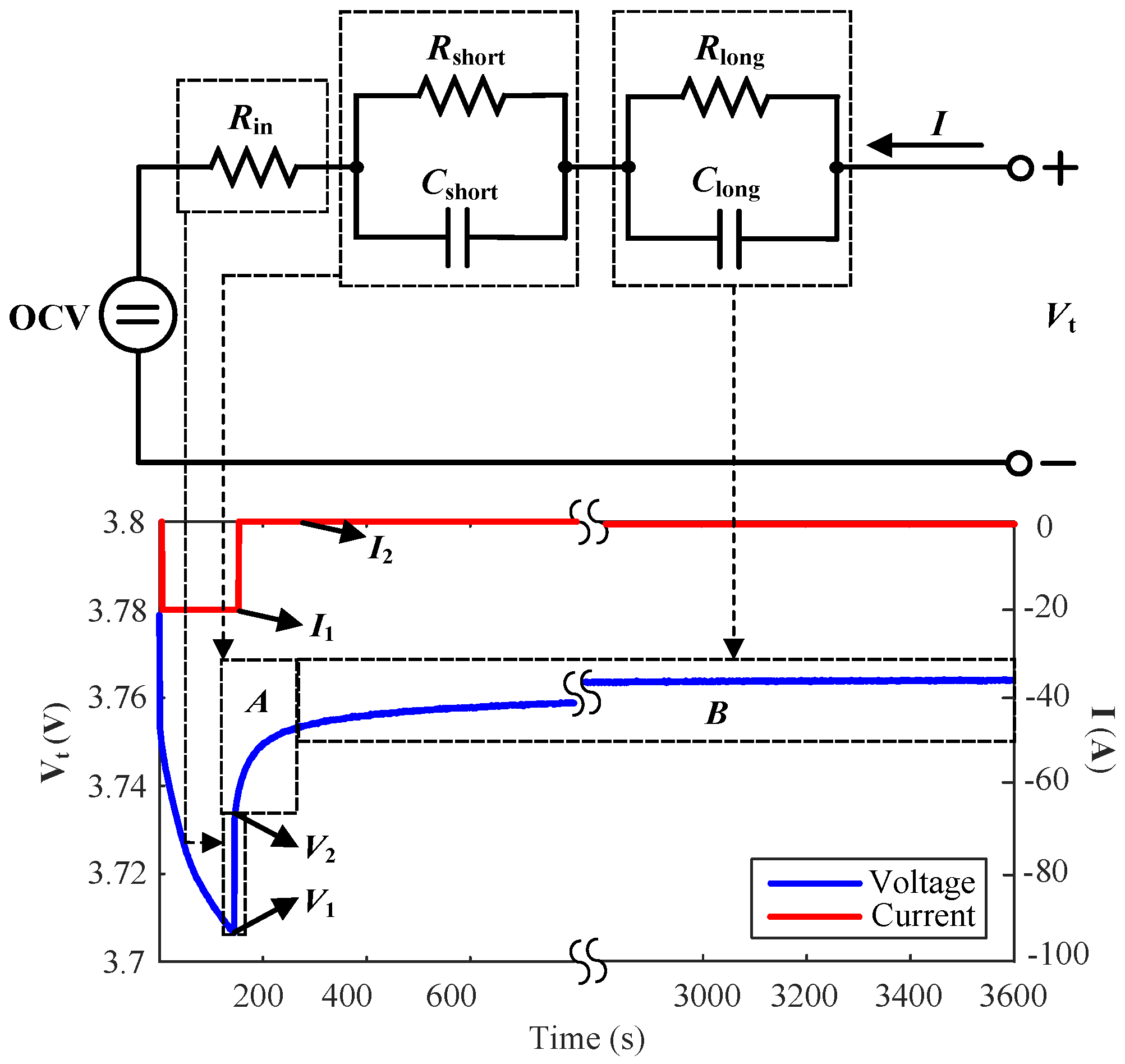
2.1. Parameter Extraction Test Design

It can be seen from Figure 1 that the second order ECM contains one OCV-SoC relationship and five impedance parameters (Rin, Rshort, Cshort, Rlong and Clong), which need to be estimated. Theoretically, all of the impedance parameters mentioned above should be multivariable functions of SoC, the C-rate of the load current (C is the amplitude of the current with which the battery can be fully discharged in 1 h), temperature and cycle numbers [39,45]. These functions not only make the parameter extraction process complex and time consuming, but also increase the computational burden of the BMS. Hence, within certain error tolerance, some relationships can be simplified or ignored. Usually, aging periods are generally in the range of months to years. While for the system-level simulations of automotive applications, the time periods of interest are typically in the range of seconds to hours or days in special cases [43,45]. Hence, the long-term aging effect is usually ignored in the parameter estimation process and handled separately in most cases [39,46].
In this paper, all of the model parameters are estimated through the discharging/charging pulse-rest test at room temperature (22 °C–25 °C). A lithium-ion polymer battery with nickel-manganese-cobalt-based cathode and graphite-based anode is under test. Its specifications are given in Table 1, and the detailed experimental steps are described as follows.
The discharging pulse-rest test starts with a fully-charged battery. In each cycle of the test, the battery is discharged at a 2% SoC step with C/2 constant current, then followed by a rest period. This cycle is repeated until the battery is fully discharged. Data points (including current, voltage, charging capacity and discharging capacity) are collected with the sampling frequency of 1 Hz. The relevant voltage and current profiles of the discharging pulse-rest test during the 66%–64% SoC interval are plotted in the bottom subfigure of Figure 1. The charging pulse-rest test is conducted similarly, that is it begins with a fully-discharged battery, then charged at a 2% SoC step with C/2 constant current and followed by a rest period. In order to eliminate the polarization voltage, the OCV values are extracted at the end of each rest period. Too short a rest time leads to a large OCV estimation error, whereas too long a rest time makes the whole test time consuming. It has been shown previously that for the lithium-ion polymer batteries, electrochemical reactions are negligible after a 2-h rest period [47,48]. Therefore, the rest time in this paper is predetermined as 2 h.

2.2. Parameter Estimation Algorithm

The electrical behavior of the ECM is expressed as the following state space formalism:
[ d V RC , short / d t d V RC , long / d t ] = [ 1 / R short C short 0 0 1 / R long C long ] [ V RC , short V RC , long ] + [ 1 / C short 1 / C long ] I
V t = O C V ( S o C ) + I R in + V RC , short + V RC , long
where Equation (1) is the state equation and Equation (2) is the output equation, VRC,short and VRC,long represent the voltages across the short-term and the long-term RC networks, respectively, OCV(SoC) is an eighth-order polynomial equation as a function of SoC, Vt is the battery terminal voltage and the positive current I represents charging. Rin represents the internal resistance; Rshort and Rlong denote the diffusion resistances; and Cshort and Clong represent the diffusion capacitances. Among them, Rin can be directly obtained from each pulse-rest cycle through Equation (3); the corresponding four variables (V1, V2, I1 and I2) are marked in the bottom subfigure of Figure 1, and the variation of identified Rin with SoC is shown in Figure 2. SoC can be calculated through Equation (4), in which Cap denotes the capacity of the battery in Ah.
R in = V 2 V 1 I 2 I 1
S o C = S o C ( 0 ) + 1 3600 C a p 0 t I ( τ ) d τ
For the CC operating scenario (I ≠ 0), the analytical solutions of Equation (1) are derived as:
{ V RC , short ( t ) = V RC , short ( 0 ) e t τ short + I R short ( 1 e t τ short ) V RC , long ( t ) = V RC , long ( 0 ) e t τ long + I R long ( 1 e t τ long )
where VRC,short(0) and VRC,long(0) are the initial voltages of corresponding RC networks and τshort = RshortCshort, τlong = RlongClong, which represent the short-term and the long-term time constants, respectively.
Substituting Equation (5) into Equation (2), the output equation is rewritten as:
V t ( t ) = O C V ( S o C ) + I R in + V RC , short ( 0 ) e t τ short + V RC , short ( 0 ) e t τ long + I R short ( 1 e t τ short ) + I R long ( 1 e t τ long )
During the rest period, where there is no current excitation (I = 0), Equation (6) can be simplified to:
V t ( t ) = O C V ( S o C ) + V RC , short ( 0 ) e t τ short + V RC , long ( 0 ) e t τ long
With the knowledge of Rin and charging/discharging OCV-SoC relationships, RC network parameters (Rshort, Cshort, Rlong and Clong) can be obtained through fitting the experimental data with relevant exponential functions, as
{ y = I R short ( 1 e t τ short ) + I R long ( 1 e t τ long ) I 0 y = V R C , short ( 0 ) e t τ short + V R C , long ( 0 ) e t τ long I = 0
where y = VtOCV(SoC)IRin. Since there only exists 2% SoC variation during each pulse-charging/discharging period, it is reasonable to make an assumption that the RC network parameters keep constant during this period. In addition, considering that the battery has converged to the steady state after a 2-h rest, VRC,short(0) and VRC,long(0) are set as zero at the beginning of the pulse-charging/discharging period.
Based on the above analysis, the RC network parameters can be estimated through fitting the experimental dataset with Equation (8). The cost function of the curve fitting method J is to minimize the sum of squared errors between the estimation results and the measured data, subjected to the following constraints:
{ J = min r , τ k = 1 n [ V t m ( t k ) V t e ( r , τ , t k ) ] 2 s . t .    R short , τ short , R long , τ long > 0
where tk is the input time sequence, n is the length of the fitted experimental dataset, r = [Rshort, Rlong], τ = [τshort, τlong], V t e is the model estimated voltage and V t m is the voltage measurements from the pulse-rest test.

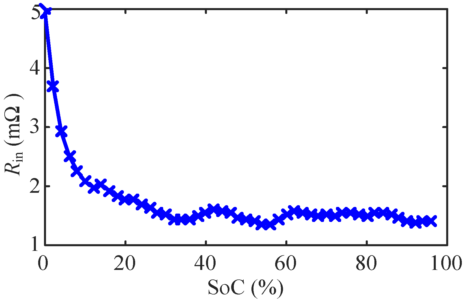
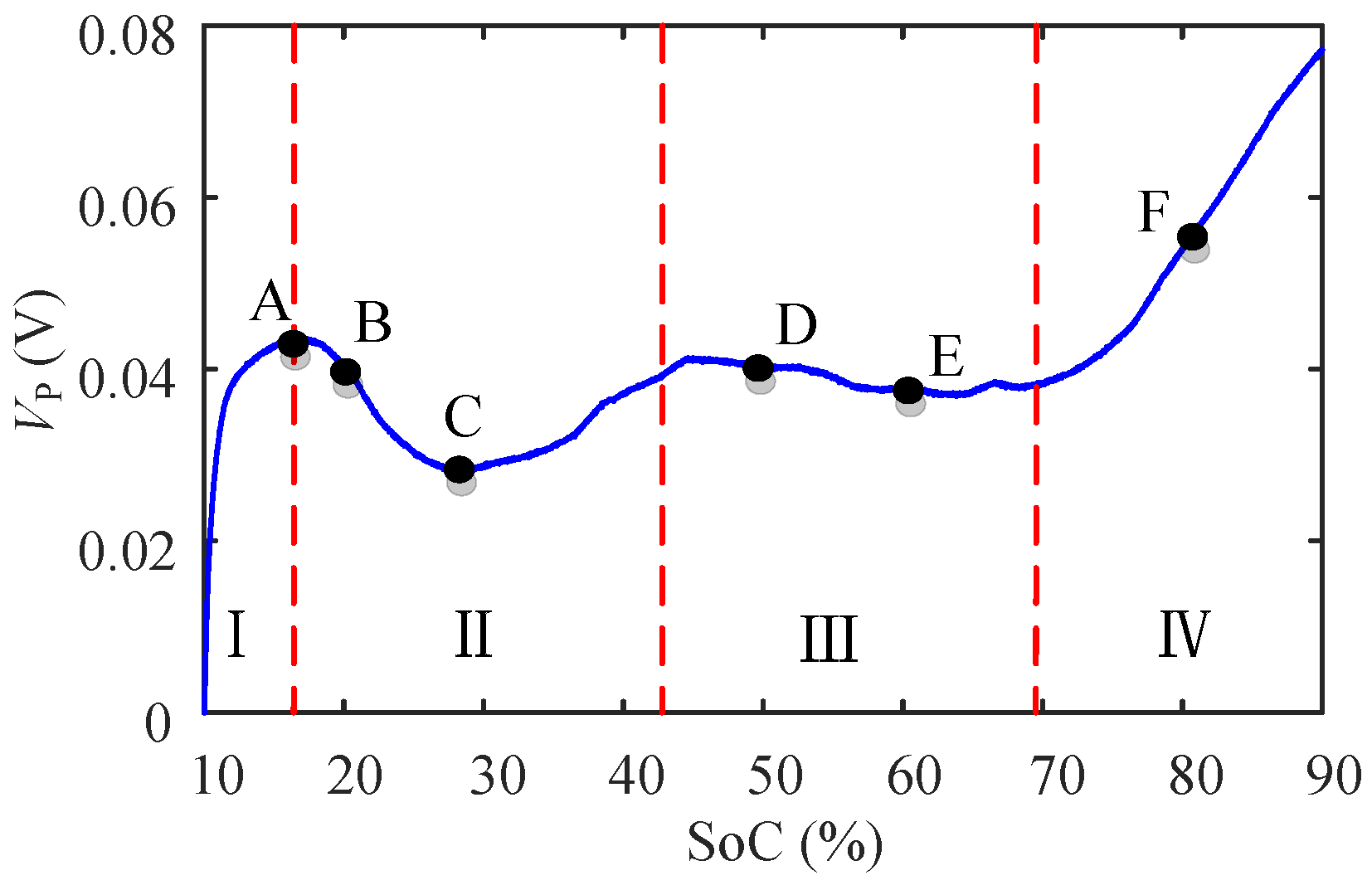
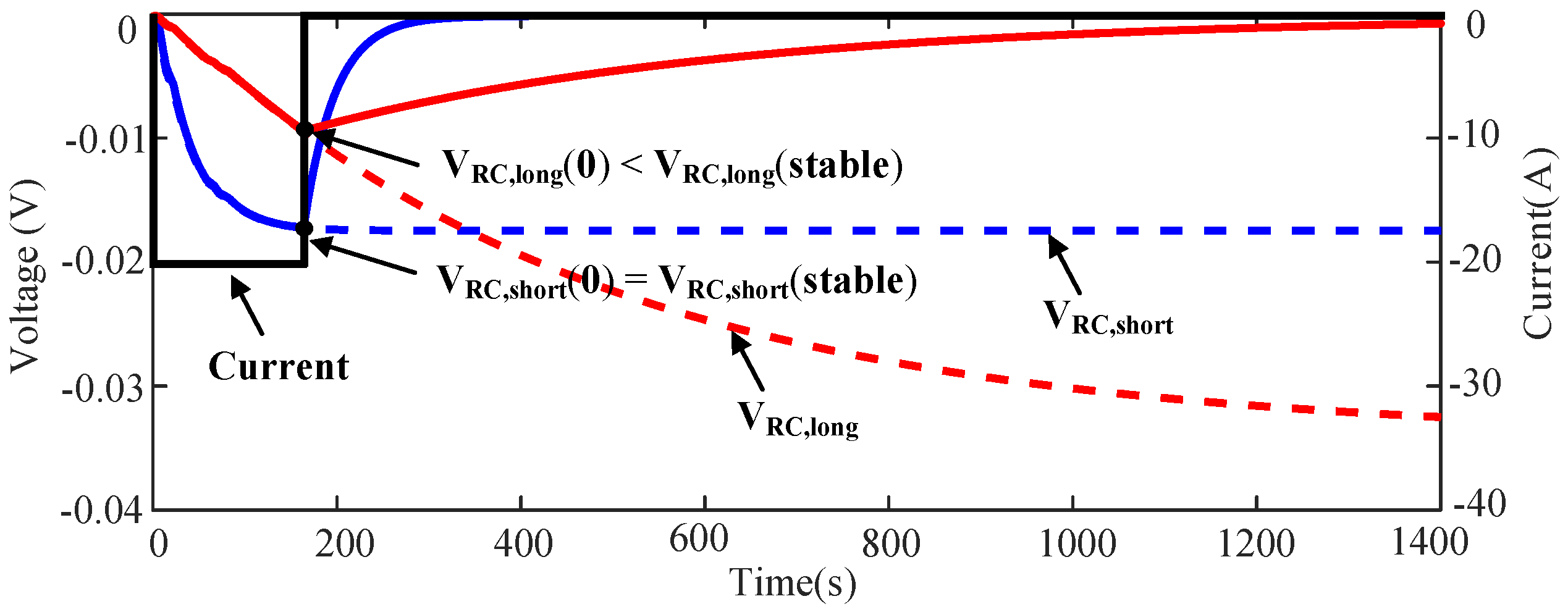
3. RC Network Parameters Estimation

Based on the Introduction in Section 1, the RC network parameters show diverse values under different operating scenarios. In HEV/EV applications, batteries usually work in two typical scenarios: the CC charging scenario and the dynamic driving scenario. In the CC charging scenario, continuous external charging currents are applied to the batteries, and the transport of ions is mainly driven by the electric field. While for the dynamical driving scenario, especially for the urban driving condition, the load current has the characteristics of discontinuous amplitude values and a wide-spread frequency spectrum. In this case, besides the electric field, the gradient in concentration is also largely responsible for the transport of ions within batteries [45]. Therefore, the RC network parameters employed in different operating scenarios should be identified through different identification approaches.

3.1. RC Network Parameters for the CC Charging Scenario

The polarization voltage (VP) is adopted to illustrate the variation of RC network parameters under the CC excitation. According to the aforementioned battery output equation, VP can be obtained as:
V P = V RC , short + V RC , long = V t O C V ( S o C ) I R in
The VP-SoC profile during the C/2 rate CC charging process is shown in Figure 3. Since in the HEV/EV application, batteries seldom work in the extremely low or high SoCs, the voltage profile from 10%–90% SoC is covered. It can be observed from Figure 3 that the polarization voltage increases dramatically in Stage I (10%–18% SoC), then it declines slowly and shows a concave shape curve in Stage II, with the local minimum value at around 30% SoC. During Stage III (40%–70% SoC), the polarization voltage becomes relatively stable. After that (70%–90% SoC), the polarization voltage rises sharply.
The variation of the polarization voltage during the above SoC range is closely related to the internal electrochemical reaction process during charging. In the initial SoC region, a relatively large amount of energy is needed to form the nucleation on the surfaces of the electrodes; thus, the polarization voltage increases quickly. Once the nuclei are formed, the following lithium ions’ removal process needs less energy. This explains the concave shape voltage curve occurring from 18% SoC to 40% SoC. While in the last charging stage, the lithium-ion concentration increases in the negative materials. Hence, a large amount of energy is needed to insert the lithium ions, which leads to the obvious growth of the polarization voltage in the high SoC region. The detailed explanation for the electrochemical reaction mechanism occurring during the CC charging process can be found in [28,32].
As mentioned in Section 2, the model parameters are estimated through fitting the measured data either from the pulse-charging period or the rest period. In order to select the proper experimental datasets that can better describe the charging characteristic of the battery, the profiles of the polarization voltage during the pulse-charging and the following rest periods, which are also calculated from Equation (10), are compared in Figure 4. Figure 4a shows the polarization voltage under the pulse-charging excitation, and Figure 4b plots the absolute values of the polarization voltage during the following rest. It can be seen from both figures that the shape of the polarization voltage curve strongly depends on the SoC. In Figure 4a, it is obvious that the final value of the polarization voltage obtained from 26%–28% SoC is the lowest, which is similar to point C in Figure 3. In addition, the final values of the voltage curves obtained from 18%–20% SoC and 50%–52% SoC are almost coincident with each other, which approximately matches the corresponding parts (point B and point D) in Figure 3. Meanwhile, the relations among the final voltage values collected from 14%–16% SoC, 60%–62% SoC and 80%–82% SoC are also identical to the relations among point A, point E and point F in Figure 3, respectively. Hence, it can be summarized from Figure 4a that the final values of the polarization voltage obtained from different pulse-charging periods are approximately consistent with the corresponding points in Figure 3. While in Figure 4b, the variation trend of the predicted stable voltage values differs greatly compared to the results in Figure 4a. This is because in the pulse-charging period, the ion migration is driven by external electric potential. While in the rest period, the transport of ions is mainly dominated by diffusion, owing to the concentration gradient. The detailed explanation of the electrochemical reactions occurring under different load current has been discussed in [21,45].
Consequently, it can be concluded that the voltage response during the pulse-charging period can better describe the characteristic of the CC charging process because of the similar current excitation.

3.2. RC Network Parameters for the Dynamic Driving Scenario

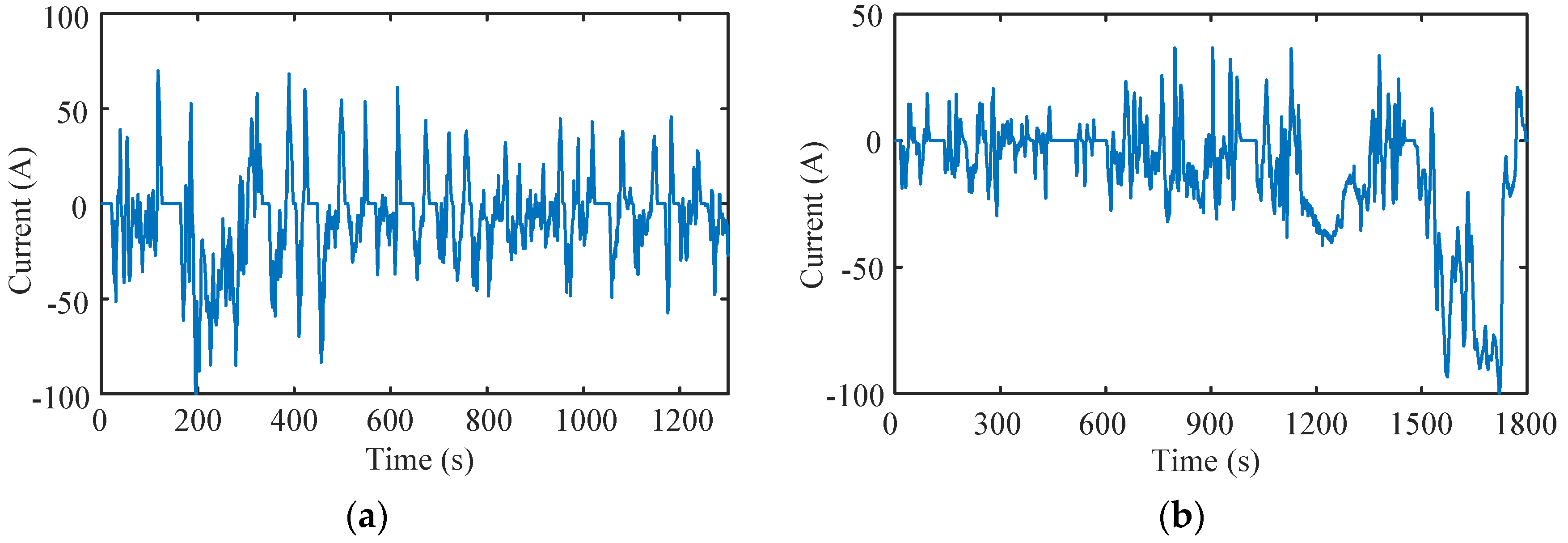
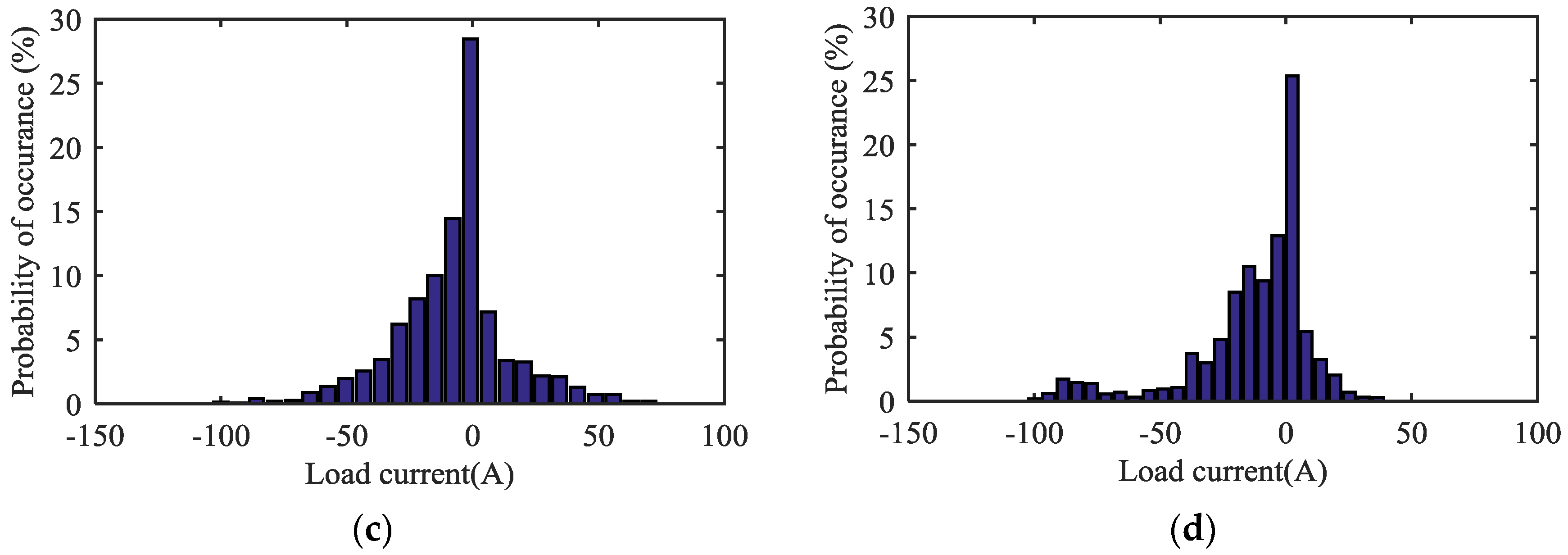
3.2.1. Typical Dynamic Driving Scenarios

For the dynamic driving scenario, especially for the urban driving scenario, vehicles accelerate and brake frequently, which cause the long lasting load current to seldom exist. There are two typical kinds of standard urban driving cycles, namely the urban dynamometer driving schedule (UDDS) and the worldwide harmonized light vehicles test procedure (WLTP), which are the American and European certification cycles, respectively. The load current profiles and the load current amplitude distributions of the two driving cycles are plotted in Figure 5. It can be observed from Figure 5a,b that both of the dynamic current profiles vary frequently over the test span. Meanwhile, from Figure 5c,d, it can be concluded that: (1) the discharging current accounts for a much larger portion, compared to the charging current during the regenerative process; (2) among the load currents, the low C-rate discharging current, particularly around zero-value amplitudes, accounts for a larger portion in both tests. Hence, the voltage response during the rest period can be employed to estimate the RC network parameters for the dynamic driving scenario.

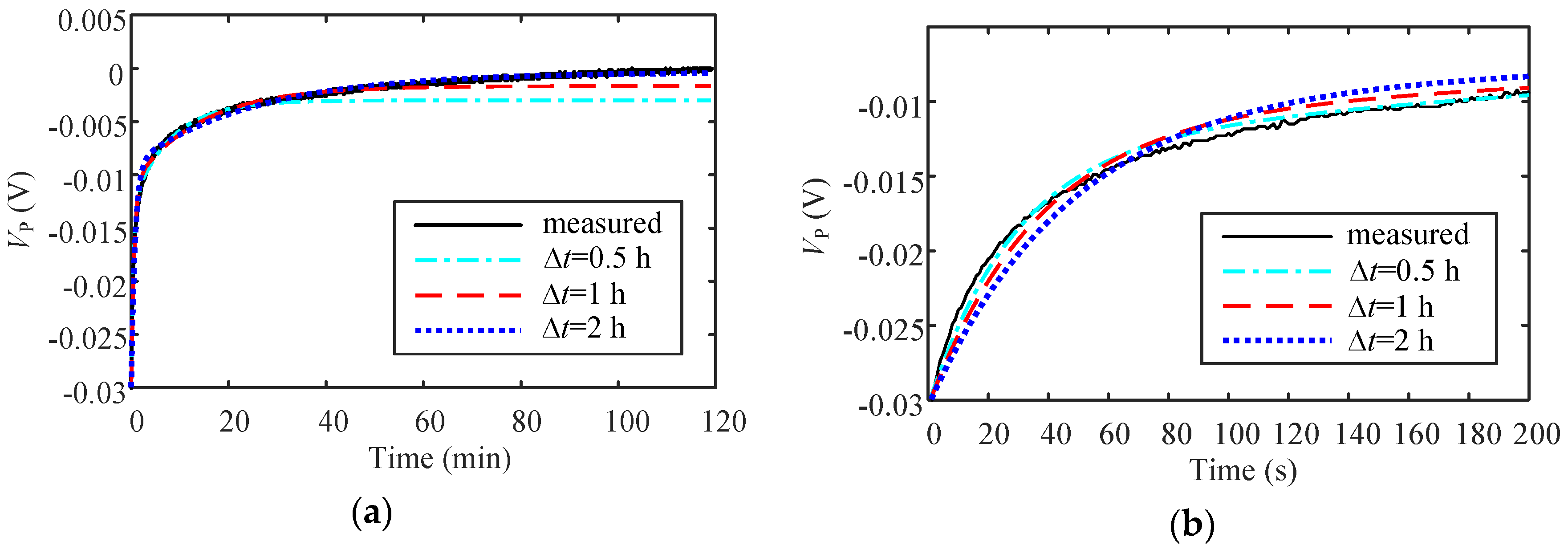
3.2.2. Determination of the Length of the Fitted Experimental Dataset

The diffusion process, which is caused by the gradient in concentration, plays a major role in the low C-rate load current and rest cases. Since the electrochemical reactions occurring during the diffusion process are very complex, these reactions can be accurately modeled as infinite series-connected RC networks with a wide range of time constants (τ1, τ2, …, τj). Usually, the values of time constants depend on the electrode thickness and the structure of the battery to a great extent, and typical time constants are in the range of seconds to minutes [45]. The second order RC network can only approximate the diffusion process by two parts: the fast dynamics part (the short-term RC network with τshort) and the slow dynamics part (the long-term RC network with τlong).
In general, the values of the two time constants are closely related to the length of the fitted experimental data ∆t. When only the initial segment of the voltage response is employed in parameter estimation, such as Part A in the bottom subfigure of Figure 1, the voltages across the shorter-term RC networks have a larger degree of variability, which means that the shorter-term RC networks have a greater impact on the initial segment of the voltage response. This in turn leads to the smaller estimated time constants and subsequently ignores the slower dynamics diffusion process. On the contrary, after the initial phase of the rest period, such as Part B in the bottom subfigure of Figure 1, the voltages across the shorter-term RC networks have converged to zero; thus, the voltage variation caused by the shorter-term RC networks is negligible. Instead, the voltages across the longer term RC networks make a remarkable contribution to the total voltage response. Subsequently, it can be inferred that the measured data show a slower varying characteristic, which represent the slower dynamics diffusion process and can be modeled by the RC networks with larger time constants. Hence, if the whole voltage response of the long time rest period is adopted, data with slower varying values will account for a large portion, which will lead to the relatively larger estimated time constants. However, too large time constants will make the model output voltage severely lag behind the actual response and result in a poor dynamic performance.
In order to further illustrate the above analysis, a third order RC network circuit is simulated in MATLAB; two equivalent time constants (τ’short and τ’long) are estimated from the different value of ∆t. In the simulation, the resistances of the three RC networks are all set as 1 mΩ, and the time constants are predetermined as τ1 = 40 s, τ2 = 200 s and τ3 = 2000 s (τ3 >> τ2> τ1). The applied excitation consists of a 400-s pulse-discharging current and a 2-h rest period, and the amplitude of the current is 20 A. Time constants estimated by different lengths of the voltage response are given in Table 2. It can be clearly seen from Table 2 that both τ’short and τ’long decrease simultaneously with the reduced value of ∆t, which is consistent with the previous analysis. Hence, to obtain the appropriate values of the time constants, ∆t should be predetermined properly, which is illustrated in detail as follows.
During ∆t, the derivative of Equation (13) with respect to τi during the rest period is expressed as:
| d V RC , i d τ i | = Δ t | V RC , i ( 0 ) | τ i 2 e Δ t τ i
where VRC,i is the voltage across the i-th RC network, i ∈ {1,2,3, …, j}, VRC,i(0) is the corresponding initial voltage, Ri is the resistance of the i-th RC network and τi is the time constant of the i-th RC network, which is subject to τ1 < τ2 < … < τj.
After the pulse-discharging period, |VRC,i(0)| can be expressed as:
| V RC , i ( 0 ) | = | I | R i ( 1 e D τ i )
where D denotes the length of the pulse-discharging period.
For the two well-separated time constants τi and τi+mi+m ≥ 10τi and 0 < m <ji), the voltage across the shorter term RC network VRC,i has a larger degree of variability when satisfying the following requirement:
| d V RC , i / d τ i | | d V RC , i + m / d τ i + m | = k
where the constant k denotes the degree of variability, and it is subject to k > 1.
Substituting Equations (11) and (12) into Equation (13), the value of ∆t can be derived as:
Δ t = ln [ R i ( 1 e D τ t ) τ i + m 2 k R i + m ( 1 e D τ t + m ) τ i 2 ] τ i τ i + m τ i + m τ i
In Equation (14), since the values of Ri and Ri+m are nearly of the same order of magnitude [39,43,46], the value of R i / R i + m can be neglected when compared to the value of τ i + m 2 / τ i 2 ; thus, ∆t can be simplified as:
Δ t = ln [ ( 1 e D τ t ) τ i + m 2 k ( 1 e D τ t + m ) τ i 2 ] τ i τ i + m τ i + m τ i
Equation (15) shows that k and τi should be determined before calculating ∆t. In the aforementioned simulation, the value of k for τ2 and τ3 can be obtained directly from Equation (13), as shown in Table 2. This indicates that when k is larger than one, the estimated τ’short and τ’long are closer to τ1 and τ2. This is because the voltage across the RC network with τ3 has a lower degree of variability, compared to those with τ1 and τ2. It can be observed from Table 2 that τ’short and τ’long are nearly stable when k is larger than 10. Hence, k is selected as 10 throughout the paper.
In order to set a proper τi in Equation (15), the discrete Fourier analysis of the load current is employed to determine the lower bandwidth limitation of the ECM. The current spectrums of UDDS and WLTP tests are shown in Figure 6. It can be observed in Figure 6a,b that there exists a large DC component (Points A and C) due to the nonzero mean value of the two current profiles. Since the characteristics of the DC component cannot be modeled by the RC circuit, they are neglected when determining the length of the fitted dataset. The major low frequency components for the two profiles are around 0.00146 Hz (point B) and 0.00138 Hz (the mean value from point D to point E), respectively. Hence, the mean value of the long-term time constant is selected as 704 s. In order to exclude the voltage variation caused by the larger time constants (larger than 10τi), the prior 1-h measured battery voltage dataset is employed to estimate the RC parameters.

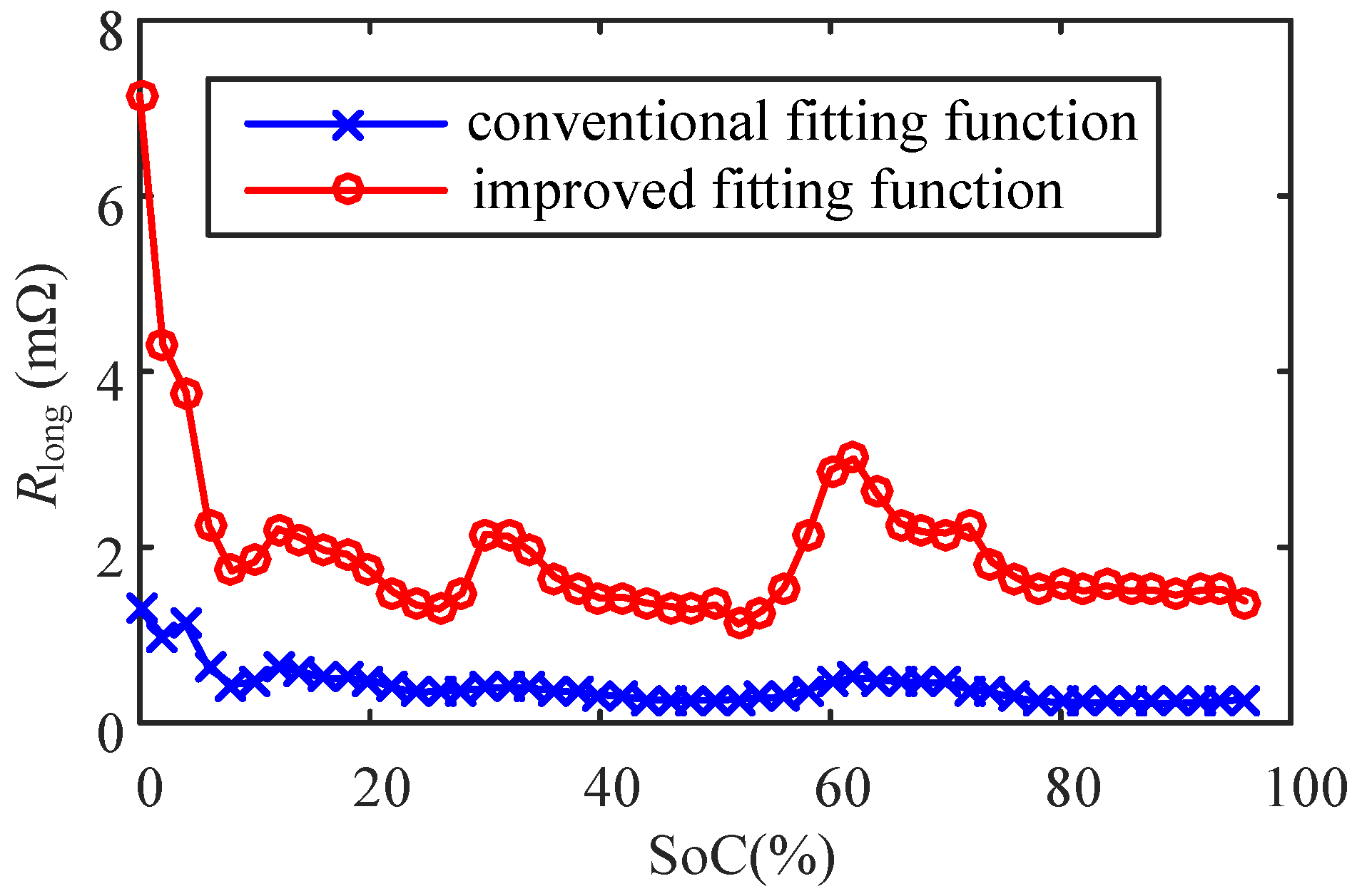
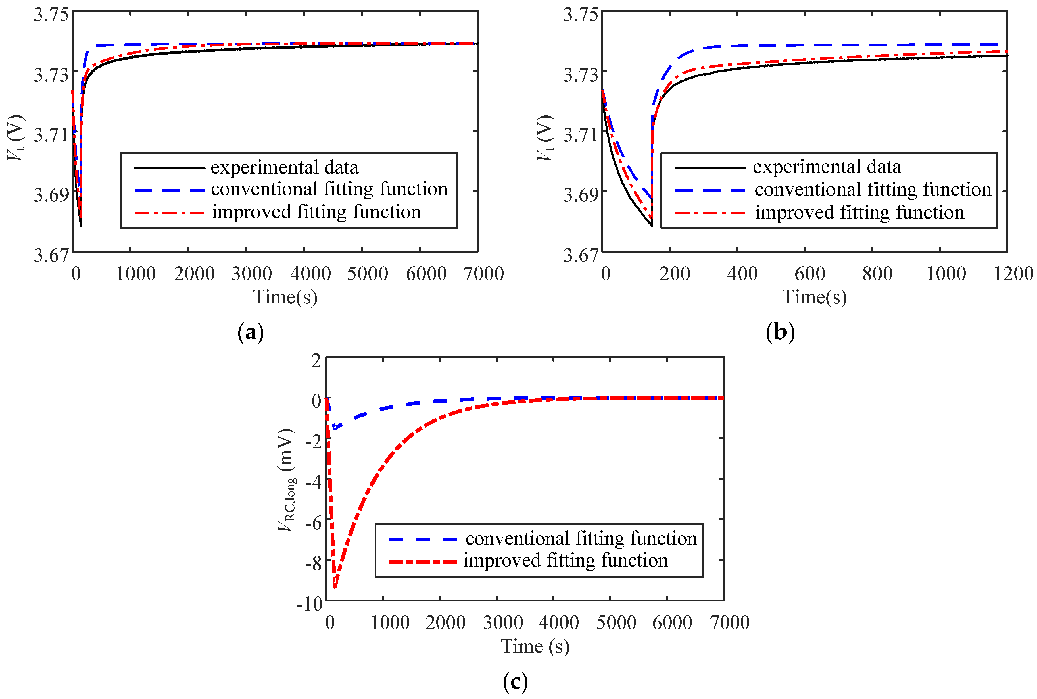
3.2.3. Improved Fitting Function

From Equations (6) and (7), it can be observed that only the initial values VRC,short(0), VRC,long(0) and time constants τshort, τlong can be obtained directly from the fitting results; thus, we should do the further computations to obtain the resistances and capacitances of RC networks.
In [37,39,40,41], two initial voltages across the RC networks are predetermined as IRshort and IRlong respectively, from which the resistances of the RC networks can be derived under the knowledge of the current value. In [49], the capacitances of the RC networks are firstly obtained from the initial voltage values. Both of the above two methods have an assumption that the capacitors of the RC networks have already converged to the steady state at the end of the pulse-discharging period.
Usually, in the parameter extraction test, in order to obtain as much data as possible at different SoC intervals, the length of the pulse-charging/discharging period is usually set as several minutes (resulting in 2% SoC variation in this paper), while the rest time is usually set as one or more hours (such as 2 h in this paper) to get an accurate OCV value. For the short-term RC network, the voltage can easily converge to the equilibrium state during the pulse-discharging process, which is shown in Figure 7. In other words, there is no current flowing through the capacitor branch of the short-term RC network during the last stage of the pulse-discharging period; thus, VRC,short(0) at the beginning of the rest period can be expressed as:
V RC , short ( 0 ) = I R short
However, for the long-term RC network, the voltage varies continuously due to a relatively large time constant, as illustrated in Figure 7. The voltage across the long-term RC network has not reached the equilibrium state at the end of the pulse-discharging period; thus, there always exists a significant proportion of the load current I ( 1 e D / τ long ) flowing through the corresponding capacitor. Consequently, VRC,long(0) at the beginning of the rest period should be written as:
V RC , long ( 0 ) = I R long ( 1 e D τ long )
where I is the value of the pulse-discharging current. Since the SoC variation in each test cycle is set as 2% in this paper, it can be assumed that the model parameters keep constant during the pulse-discharging period.

4. Experimental Results and Discussions

4.1. RC Network Parameter Estimation Results

Based on the aforementioned analysis in Section 3.1, for the case of the CC charging scenario, the charging pulse-rest test is implemented firstly. The parameters are estimated from the voltage response of the pulse-charging period, and the estimation results are shown in Figure 8. Figure 8a plots two estimated time constants; it can be seen that the general order of the magnitude of the short-term time constant is 10 s; it fluctuates greatly when the SoC changes, especially in the middle SoC region, while the order of the magnitude of the long-term time constant is 100 s; it is relatively flat during the whole SoC region. Figure 8b plots two estimated resistances; it can be observed that in the middle SoC range, the short-term resistance has a larger value, which means that the voltage across the short-term RC network accounts for more weight during this period. Hence, it can be observed from Figure 3 and Figure 8b that the variation tendencies of the polarization voltage and the short-term resistance are similar during the middle SoC range. At the end of the charging process, the short-term resistance decreases and stabilizes around a very small value, while the long-term resistance increases almost linearly after 60% SoC, leading to a similar variation tendency of the polarization voltage, compared to the corresponding part in Figure 3. Hence, it can be concluded that the long-term diffusion process plays a major role in this stage.
For the case of the dynamic driving scenario, the discharging pulse-rest test is implemented, and the data from the rest periods are adopted in the parameter estimation. According to the analysis in Section 3.2.2, different time constants will be obtained from the fitted experimental datasets in different lengths. Firstly, in order to compare the best fit performances for the measured datasets in different lengths, the measured battery terminal voltage response at 60% SoC during a 2-h rest period is adopted, and the curve fitting results are shown in Figure 9. It can be observed from Figure 9a that the fitting result of the whole measured voltage response shows a better performance during most of the rest period, especially in the equilibrium state. Whereas for the performance of the first 200 s, the fitting result through the prior 0.5-h measured voltage response yields less errors, which is illustrated in Figure 9b. Parameter estimation results in Figure 10 show the time constants estimated from the measured voltage dataset in different lengths, ranging from 30 min–2 h with a 30-min interval. It can be observed that the time constants, both for the long term and the short term, increase simultaneously when the length of the fitted dataset increases. In addition, by comparing Figure 10 with Figure 8a, it can be concluded that the time constants applied in the CC charging scenario and the dynamic driving scenario show different variation tendencies. Hence, it is essential to adopt different sets of model parameters for different operating scenarios.
After determining the length of the fitted experimental dataset, we can subsequently obtain the resistances. Figure 11 shows the Rlong estimation results by the conventional fitting function and the improved fitting function. It can be concluded from Figure 11 that the Rlong estimated by the conventional fitting function is generally less than the one estimated by the improved fitting function, because it neglects the ( 1 e D / τ long ) part. In order to demonstrate the advantage of the improved fitting function, data from the 20th cycle of the discharging pulse-rest test are adopted. In this cycle, SoC changes from 62% to 60% during the pulse-discharging period, then keeps the value of 60% during the following rest period. The current profile of the 20th discharging pulse-rest test is applied on the ECM MATLAB/SIMULINK model as an excitation. Figure 12a,b shows the model output voltage responses with two sets of estimated model parameters. It can be seen that the model with parameters estimated by the proposed fitting function outputs better estimation results. The lower voltage error is mainly contributed by the higher voltage drop across the long-term RC network, as plotted in Figure 12c. In addition, the root mean square errors (RMSEs) between the measured voltage and the model output voltage at different SoCs are given in Table 3. It can also be seen that the model parameters estimated by the proposed fitting function show a better performance for a wide range of SoC.

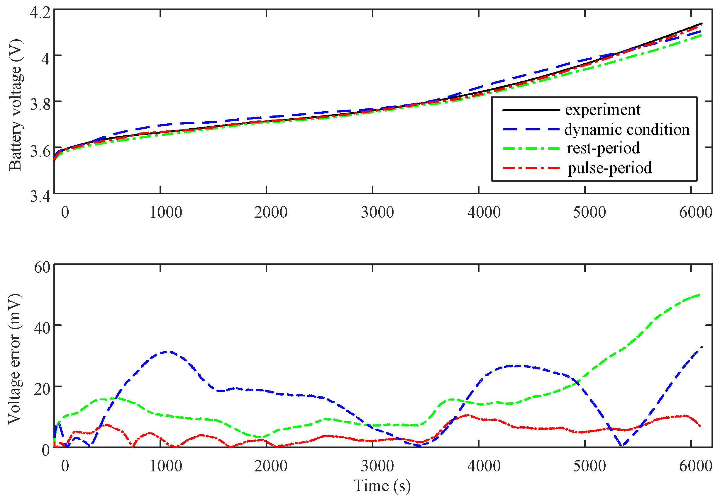
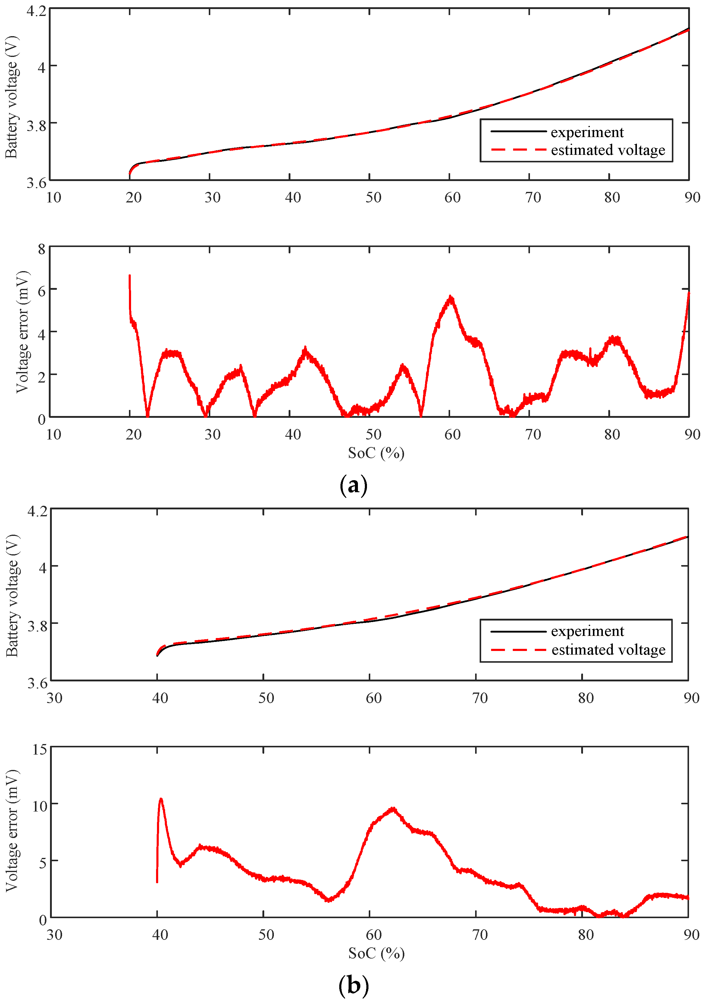
4.2. Model Verification

In this paper, the CC charging test and the consecutive UDDS test, which respectively represent two typical operating scenarios in HEV/EV applications, are conducted separately to verify the effectiveness of the model. For the charging condition, the battery is charged from 10%–90% SoC. The typical charging current in practice varies from C/8 to 2C [50], and a C/2 rate current is employed in the charging test. The consecutive UDDS test starts from 90% SoC to 20% SoC, with a 10-min rest period in between to simulate a short parking time. In the real application, a specific set of parameters can be selected by the characteristics of the measured load current. For example, if the values of the current are approximately constant over a certain time interval, parameters estimated from the data in the pulse-charging periods are employed. On the other hand, parameters estimated from the data in the rest periods are employed when the load current shows the characteristics of high dynamics over a certain time interval.
Firstly, for the CC charging scenario, three model outputs and measured battery terminal voltage curves are plotted in Figure 13, and the corresponding RMSEs are given in Table 4. It can be observed that during the whole charging process, the model with parameters estimated from the data in pulse-charging periods outputs a voltage curve matching the measured curve better because of considering the continuous external electric driving forces. However, parameters estimated from the data in the rest periods result in relatively larger errors, especially in the high SoC region. In addition, during most part of the charging period, the model with parameters used in the dynamic driving scenarios outputs a voltage higher than the experimental voltage. Comparing the corresponding curves in Figure 8b and Figure 11, it can be deduced that the higher estimated voltage is mainly caused by the larger value of estimated Rlong, especially during the middle range of the SoC region.
In order to verify the robustness of the proposed parameter estimation method, the CC charging voltage profiles at different initial SoC are plotted in Figure 14. This shows that the estimated voltage curves match well with the measurement voltage curves, despite the different initial SoC.
Secondly, in order to demonstrate the improvement of the proposed battery modelling approach during the dynamic driving scenario, the model and experimental voltage outputs in the consecutive UDDS validation are plotted in Figure 15a, the corresponding calculated SoC profile is shown in Figure 15b, and the detailed figure from 10,000 s to 12,000 s is plotted in Figure 15c. The RMSE of the aforementioned estimation methods during the whole consecutive UDDS test are also shown in Table 5. Figure 15b shows that the consecutive UDDS test is started from 90% SoC, and terminated when the value of SoC drops below 20%. It can be observed from Figure 15c that parameters estimated by the improved fitting function generally demonstrate a better performance, especially during the dynamic period (ranging from 10,000 s to 11,400 s), because considering the unsaturated phenomenon of the long-term RC network. It can also be concluded that the model containing parameters estimated by the prior 1-h experimental data from the rest period gives voltage output with the least error, especially during the short-time rest period. In addition, it can be seen from Figure 5a that there exists a relatively long-time and high C-rate discharging current in the UDDS cycle approximately ranging from 150 s to 300 s. Since larger time constants are obtained from the data of the whole rest period, this causes the corresponding voltage output not to recover fast after a relatively long-time discharging current, which leads to an offset of voltage errors in comparison to the voltage error caused by the proposed approach.

5. Conclusions

In this paper, an advanced battery parameter estimation method based on two general operating scenarios in HEV/EV applications is proposed. Firstly, the second order ECM is employed, and the model parameter extraction process is described in detail. Considering the typical operating scenarios in HEV/EV applications, namely the CC charging scenario and the dynamic driving scenario, two sets of model parameters are extracted from the charging/discharging pulse-rest tests. Specifically, voltage responses of the pulse-charging phases are selected to estimate model parameters applied in the CC charging scenario. For the dynamic driving scenario, the model parameters are identified through the measured data from the rest period. Instead of employing the data from the whole rest period, only the prior portion of the collected data is selected, and the length of the fitted data is determined by the frequency spectrum analysis of the load current under two typical urban driving conditions. In addition, an unsaturated phenomenon caused by the long-term RC network is analyzed in detail, and subsequently, an improved fitting equation with more accurate initial voltage expression of the RC network is adopted. Finally, verification tests simulating the CC charging scenario and the dynamic driving scenario are conducted, respectively, and comparisons between the conventional and the proposed battery parameter estimation methods are given. Experimental results show that in both cases, the voltage profiles predicted from the proposed model show a better conformity to the experimental data.
It is important to note that the proposed battery parameter estimation method for the dynamic driving scenario only considers the typical urban driving conditions at room temperature. However, the characteristics of the load current under the other special conditions (such as the highway driving condition and the extremely cold condition) will be obviously different. For the future work, the influence caused by different C-rates of the current profiles, bandwidths of the current profiles and temperature effects will be considered, and the parameter extraction test will be modified accordingly.

Acknowledgments

The authors would like to acknowledge the funding support from the China Scholarship Council (CSC); the U.S. DOE Graduate Automotive Technology Education (GATE) Center of Excellence; and Nanjing Golden Dragon Bus Co., Ltd.

Author Contributions

Jufeng Yang handled the technical modeling, drafted and revised the manuscript. Bing Xia revised the manuscript. Jufeng Yang and Bing Xia designed the experiments and analyzed the data. Yunlong Shang participated in the experiment. Wenxin Huang revised the manuscript. Chris Mi contributed the experiment platform, gave great suggestions and polished the manuscript.

Conflicts of Interest

The authors declare no conflict of interest.

References

  1. Xiong, R.; Sun, F.; Chen, Z.; He, H. A data-driven multi-scale extended kalman filtering based parameter and state estimation approach of lithium-ion olymer battery in electric vehicles. Appl. Energy 2014, 113, 463–476. [Google Scholar] [CrossRef]
  2. Zou, Z.; Xu, J.; Mi, C.; Cao, B.; Chen, Z. Evaluation of model based state of charge estimation methods for lithium-ion batteries. Energies 2014, 7, 5065–5082. [Google Scholar] [CrossRef]
  3. Shang, Y.; Zhang, C.; Cui, N.; Guerrero, J.M. A cell-to-cell battery equalizer with zero-current switching and zero-voltage gap based on quasi-resonant lc converter and boost converter. IEEE Trans. Power Electron. 2015, 30, 3731–3747. [Google Scholar] [CrossRef]
  4. Xia, B.; Mi, C. A fault-tolerant voltage measurement method for series connected battery packs. J. Power Sources 2016, 308, 83–96. [Google Scholar] [CrossRef]
  5. Sun, F.; Xiong, R.; He, H. A systematic state-of-charge estimation framework for multi-cell battery pack in electric vehicles using bias correction technique. Appl. Energy 2016, 162, 1399–1409. [Google Scholar] [CrossRef]
  6. Xia, B.; Shang, Y.; Nguyen, T.; Mi, C. A correlation based fault detection method for short circuits in battery packs. J. Power Sources 2017, 337, 1–10. [Google Scholar] [CrossRef]
  7. Salameh, M.; Schweitzer, B.; Sveum, P.; Al-Hallaj, S.; Krishnamurthy, M. Online temperature estimation for phase change composite-18650 lithium ion cells based battery pack. In Proceedings of the 2016 IEEE Applied Power Electronics Conference and Exposition (APEC), Long Beach, CA, USA, 20–24 March 2016; pp. 3128–3133.
  8. Seaman, A.; Dao, T.-S.; McPhee, J. A survey of mathematics-based equivalent-circuit and electrochemical battery models for hybrid and electric vehicle simulation. J. Power Sources 2014, 256, 410–423. [Google Scholar] [CrossRef]
  9. Zou, Y.; Hu, X.; Ma, H.; Li, S.E. Combined state of charge and state of health estimation over lithium-ion battery cell cycle lifespan for electric vehicles. J. Power Sources 2015, 273, 793–803. [Google Scholar] [CrossRef]
  10. Wei, Z.; Tseng, K.J.; Wai, N.; Lim, T.M.; Skyllas-Kazacos, M. Adaptive estimation of state of charge and capacity with online identified battery model for vanadium redox flow battery. J. Power Sources 2016, 332, 389–398. [Google Scholar] [CrossRef]
  11. He, H.; Xiong, R.; Guo, H.; Li, S. Comparison study on the battery models used for the energy management of batteries in electric vehicles. Energy Convers. Manag. 2012, 64, 113–121. [Google Scholar] [CrossRef]
  12. He, H.; Zhang, X.; Xiong, R.; Xu, Y.; Guo, H. Online model-based estimation of state-of-charge and open-circuit voltage of lithium-ion batteries in electric vehicles. Energy 2012, 39, 310–318. [Google Scholar] [CrossRef]
  13. Nejad, S.; Gladwin, D.; Stone, D. A systematic review of lumped-parameter equivalent circuit models for real-time estimation of lithium-ion battery states. J. Power Sources 2016, 316, 183–196. [Google Scholar] [CrossRef]
  14. Xia, B.; Zhao, X.; De Callafon, R.; Garnier, H.; Nguyen, T.; Mi, C. Accurate lithium-ion battery parameter estimation with continuous-time system identification methods. Appl. Energy 2016, 179, 426–436. [Google Scholar] [CrossRef]
  15. Pérez, G.; Garmendia, M.; Reynaud, J.F.; Crego, J.; Viscarret, U. Enhanced closed loop state of charge estimator for lithium-ion batteries based on extended kalman filter. Appl. Energy 2015, 155, 834–845. [Google Scholar] [CrossRef]
  16. Chen, Z.; Fu, Y.; Mi, C.C. State of charge estimation of lithium-ion batteries in electric drive vehicles using extended kalman filtering. IEEE Trans. Veh. Technol. 2013, 62, 1020–1030. [Google Scholar] [CrossRef]
  17. Sun, F.; Xiong, R. A novel dual-scale cell state-of-charge estimation approach for series-connected battery pack used in electric vehicles. J. Power Sources 2015, 274, 582–594. [Google Scholar] [CrossRef]
  18. Li, K.; Tseng, K.J. An equivalent circuit model for state of energy estimation of lithium-ion battery. In Proceedings of the 2016 IEEE Applied Power Electronics Conference and Exposition (APEC), Long Beach, CA, USA, 20–24 March 2016; pp. 3422–3430.
  19. Fuller, T.F.; Doyle, M.; Newman, J. Relaxation phenomena in lithium-ion-insertion cells. J. Electrochem. Soc. 1994, 141, 982–990. [Google Scholar] [CrossRef]
  20. Smith, K.A. Electrochemical Modeling, Estimation and Control of Lithium Ion Batteries. Ph.D. Thesis, The Pennsylvania State University, State College, PA, USA, 2006. [Google Scholar]
  21. Park, M.; Zhang, X.; Chung, M.; Less, G.B.; Sastry, A.M. A review of conduction phenomena in Li-ion batteries. J. Power Sources 2010, 195, 7904–7929. [Google Scholar] [CrossRef]
  22. Karden, E.; Buller, S.; De Doncker, R.W. A method for measurement and interpretation of impedance spectra for industrial batteries. J. Power Sources 2000, 85, 72–78. [Google Scholar] [CrossRef]
  23. Thele, M.; Bohlen, O.; Sauer, D.U.; Karden, E. Development of a voltage-behavior model for nimh batteries using an impedance-based modeling concept. J. Power Sources 2008, 175, 635–643. [Google Scholar] [CrossRef]
  24. Buller, S.; Thele, M.; De Doncker, R.; Karden, E. Impedance-based simulation models of supercapacitors and Li-ion batteries for power electronic applications. IEEE Trans. Ind. Appl. 2005, 41, 742–747. [Google Scholar] [CrossRef]
  25. Waag, W.; Käbitz, S.; Sauer, D.U. Experimental investigation of the lithium-ion battery impedance characteristic at various conditions and aging states and its influence on the application. Appl. Energy 2013, 102, 885–897. [Google Scholar] [CrossRef]
  26. Howey, D.A.; Mitcheson, P.D.; Yufit, V.; Offer, G.J.; Brandon, N.P. Online measurement of battery impedance using motor controller excitation. IEEE Trans. Veh. Technol. 2014, 63, 2557–2566. [Google Scholar] [CrossRef]
  27. Zheng, Y.; Lu, L.; Han, X.; Li, J.; Ouyang, M. Lifepo 4 battery pack capacity estimation for electric vehicles based on charging cell voltage curve transformation. J. Power Sources 2013, 226, 33–41. [Google Scholar] [CrossRef]
  28. Nakayama, M.; Iizuka, K.; Shiiba, H.; Baba, S.; Nogami, M. Asymmetry in anodic and cathodic polarization profile for LiFePO4 positive electrode in rechargeable Li ion battery. J. Ceram. Soc. Jpn. 2011, 119, 692–696. [Google Scholar] [CrossRef]
  29. Musio, M.; Damiano, A. A simplified charging battery model for smart electric vehicles applications. In Proceedings of the 2014 IEEE International Energy Conference (ENERGYCON), Dubrovnik, Croatia, 13–16 May 2014; pp. 1357–1364.
  30. Tsang, K.; Sun, L.; Chan, W. Identification and modelling of lithium ion battery. Energy Convers. Manag. 2010, 51, 2857–2862. [Google Scholar] [CrossRef]
  31. Yao, L.W.; Aziz, J.; Kong, P.Y.; Idris, N.; Alsofyani, I. Modeling of lithium titanate battery for charger design. In Proceedings of the 2014 IEEE Australasian Universities Power Engineering Conference (AUPEC), Perth, Australia, 28 Sepember–1 October 2014; pp. 1–5.
  32. Jiang, J.; Liu, Q.; Zhang, C.; Zhang, W. Evaluation of acceptable charging current of power Li-ion batteries based on polarization characteristics. IEEE Trans. Ind. Electron. 2014, 61, 6844–6851. [Google Scholar] [CrossRef]
  33. Kim, N.; Ahn, J.-H.; Kim, D.-H.; Lee, B.-K. Adaptive loss reduction charging strategy considering variation of internal impedance of lithium-ion polymer batteries in electric vehicle charging systems. In Proceedings of the 2016 IEEE Applied Power Electronics Conference and Exposition (APEC), Long Beach, CA, USA, 20–24 March 2016; pp. 1273–1279.
  34. Chen, Z.; Xia, B.; Mi, C.C.; Xiong, R. Loss-minimization-based charging strategy for lithium-ion battery. IEEE Trans. Ind. Appl. 2015, 51, 4121–4129. [Google Scholar] [CrossRef]
  35. Rao, R.; Vrudhula, S.; Rakhmatov, D.N. Battery modeling for energy aware system design. Computer 2003, 36, 77–87. [Google Scholar]
  36. Fleischer, C.; Waag, W.; Heyn, H.-M.; Sauer, D.U. On-line adaptive battery impedance parameter and state estimation considering physical principles in reduced order equivalent circuit battery models: Part 1. Requirements, critical review of methods and modeling. J. Power Sources 2014, 260, 276–291. [Google Scholar] [CrossRef]
  37. Schweighofer, B.; Raab, K.M.; Brasseur, G. Modeling of high power automotive batteries by the use of an automated test system. IEEE Trans. Instrum. Meas. 2003, 52, 1087–1091. [Google Scholar] [CrossRef]
  38. Castano, S.; Gauchia, L.; Voncila, E.; Sanz, J. Dynamical modeling procedure of a Li-ion battery pack suitable for real-time applications. Energy Convers. Manag. 2015, 92, 396–405. [Google Scholar] [CrossRef]
  39. Chen, M.; Rincon-Mora, G.A. Accurate electrical battery model capable of predicting runtime and iv performance. IEEE Trans. Energy Convers. 2006, 21, 504–511. [Google Scholar] [CrossRef]
  40. Baronti, F.; Fantechi, G.; Leonardi, E.; Roncella, R.; Saletti, R. Enhanced model for lithium-polymer cells including temperature effects. In Proceedings of the IECON 2010—36th Annual Conference on IEEE Industrial Electronics Society, Glendale, AZ, USA, 7–10 November 2010; pp. 2329–2333.
  41. Lam, L.; Bauer, P.; Kelder, E. A practical circuit-based model for li-ion battery cells in electric vehicle applications. In Proceedings of the 2011 IEEE 33rd International Telecommunications Energy Conference (INTELEC), Amsterdam, The Netherlands, 9–13 October 2011; pp. 1–9.
  42. Hu, Y.; Wang, Y.-Y. Two time-scaled battery model identification with application to battery state estimation. IEEE Trans. Control Syst. Technol. 2015, 23, 1180–1188. [Google Scholar] [CrossRef]
  43. Li, J.; Mazzola, M.S. Accurate battery pack modeling for automotive applications. J. Power Sources 2013, 237, 215–228. [Google Scholar] [CrossRef]
  44. Widanage, W.; Barai, A.; Chouchelamane, G.; Uddin, K.; McGordon, A.; Marco, J.; Jennings, P. Design and use of multisine signals for Li-ion battery equivalent circuit modelling. Part 1: Signal design. J. Power Sources 2016, 324, 70–78. [Google Scholar] [CrossRef]
  45. Jossen, A. Fundamentals of battery dynamics. J. Power Sources 2006, 154, 530–538. [Google Scholar] [CrossRef]
  46. Hentunen, A.; Lehmuspelto, T.; Suomela, J. Time-domain parameter extraction method for thévenin-equivalent circuit battery models. IEEE Trans. Energy Convers. 2014, 29, 558–566. [Google Scholar] [CrossRef]
  47. Petzl, M.; Danzer, M.A. Advancements in OCV measurement and analysis for lithium-ion batteries. IEEE Trans. Energy Convers. 2013, 28, 675–681. [Google Scholar] [CrossRef]
  48. Barai, A.; Widanage, W.D.; Marco, J.; McGordon, A.; Jennings, P. A study of the open circuit voltage characterization technique and hysteresis assessment of lithium-ion cells. J. Power Sources 2015, 295, 99–107. [Google Scholar] [CrossRef]
  49. Hariharan, K.S.; Kumar, V.S. A nonlinear equivalent circuit model for lithium ion cells. J. Power Sources 2013, 222, 210–217. [Google Scholar] [CrossRef]
  50. Gong, X.; Xiong, R.; Mi, C.C. A data-driven bias-correction-method-based lithium-ion battery modeling approach for electric vehicle applications. IEEE Trans. Ind. Appl. 2016, 52, 1759–1765. [Google Scholar]
Figure 1. The second order equivalent circuit model (ECM). OCV, open circuit voltage.
Energies 10 00005 g001
Figure 2. Rin variation with different state of charge (SoC).
Energies 10 00005 g002
Figure 3. VP versus SoC under constant-current (CC) charging.
Energies 10 00005 g003
Figure 4. (a) The profiles of VP at different SoC intervals during the pulse-charging period; (b) the profiles of |VP| at different SoC points during the rest period.
Energies 10 00005 g004
Figure 5. (a) The load current profile of the urban dynamometer driving schedule (UDDS) test; (b) the load current profile of the worldwide harmonized light vehicles test procedure (WLTP) test; (c) the load current amplitude distribution of the UDDS test; (d) the load current amplitude distribution of the WLTP test.
Energies 10 00005 g005aEnergies 10 00005 g005b
Figure 6. The spectral analysis of the load current: (a) the urban dynamometer driving schedule (UDDS) test; (b) the worldwide harmonized light vehicles test procedure (WLTP) test.
Energies 10 00005 g006
Figure 7. The voltage curve of RC networks during one cycle of the discharging pulse-rest test.
Energies 10 00005 g007
Figure 8. Parameter estimation results for the constant-current (CC) charging scenario: (a) time constant; (b) resistance.
Energies 10 00005 g008
Figure 9. Curve fitting results of VP during the rest period of the discharging pulse-rest test at 60% SoC: (a) the overall result; (b) a close look at the transient part at the beginning.
Energies 10 00005 g009
Figure 10. Time constant estimation results with different lengths of the experimental dataset: (a) τshort; (b) τlong.
Energies 10 00005 g010
Figure 11. Rlong estimation results.
Energies 10 00005 g011
Figure 12. Voltage curves of one cycle of the discharging pulse-rest test (62%–60%): (a) the overview; (b) a close look; (c) the voltage across the long-term RC network.
Energies 10 00005 g012
Figure 13. Verification results of different parameter estimation methods under the CC charging test.
Energies 10 00005 g013
Figure 14. CC charging voltage profiles at different initial SoC: (a) initial SoC = 20%; (b) initial SoC = 40%.
Energies 10 00005 g014
Figure 15. Verification results of different parameter estimation methods under the UDDS tests: (a) The overall look; (b) The calculated SoC profile (c) The close look.
Energies 10 00005 g015
Table 1. Specification of the tested battery.
Charge Capacity40.99 Ah
Discharge capacity40.89 Ah
Nominal voltage3.7 V
Charge cutoff voltage4.2 V
Discharge cutoff voltage2.7 V
Table 2. Equivalent time constant estimation results with different values of ∆t.
t (s)720036001800140012001000900850800
τ’short (s)88.6767.1848.5345.1043.7442.5942.0841.8341.63
τ’long (s)971.0484.3284.4256.7245.3235.3230.9228.8226.8
k 14.049 × 10−124.395 × 10−50.14480.87592.1545.2998.31110.4113.03
1 k represents the degree of resistor-capacitor (RC) voltage variability; the detailed expression can referred to in Equation (13).
Table 3. Comparison of RMSE at different SoC.
SoC (%) 102030405060708090
RMSE (mV)Conventional fitting function1.8021.7142.1671.5401.2682.8032.4161.5581.444
Improved fitting function0.76580.75820.97070.76430.50001.2021.2420.71040.6482
Table 4. RMSE of model voltage estimation under the CC charging test.
Modeling MethodsDynamic ConditionRest-PeriodPulse-Period
RMSE (mV)18.4119.765.448
Table 5. RMSE of the model voltage estimation under the urban dynamometer driving schedule (UDDS) test.
Modeling MethodsConventionalImproved-2 hImproved-1 h
RMSE (mV)8.5046.3294.244

