
Towards Operational Detection of Forest Ecosystem Changes in Protected Areas


 , ,
, ,
Abstract
:1. Introduction
1.1. Change Detection Techniques
1.2. Change Detection with VHR Images
1.3. CCA Based Scenario Technique at VHR and HR
2. Materials and Methods
2.1. Site Description
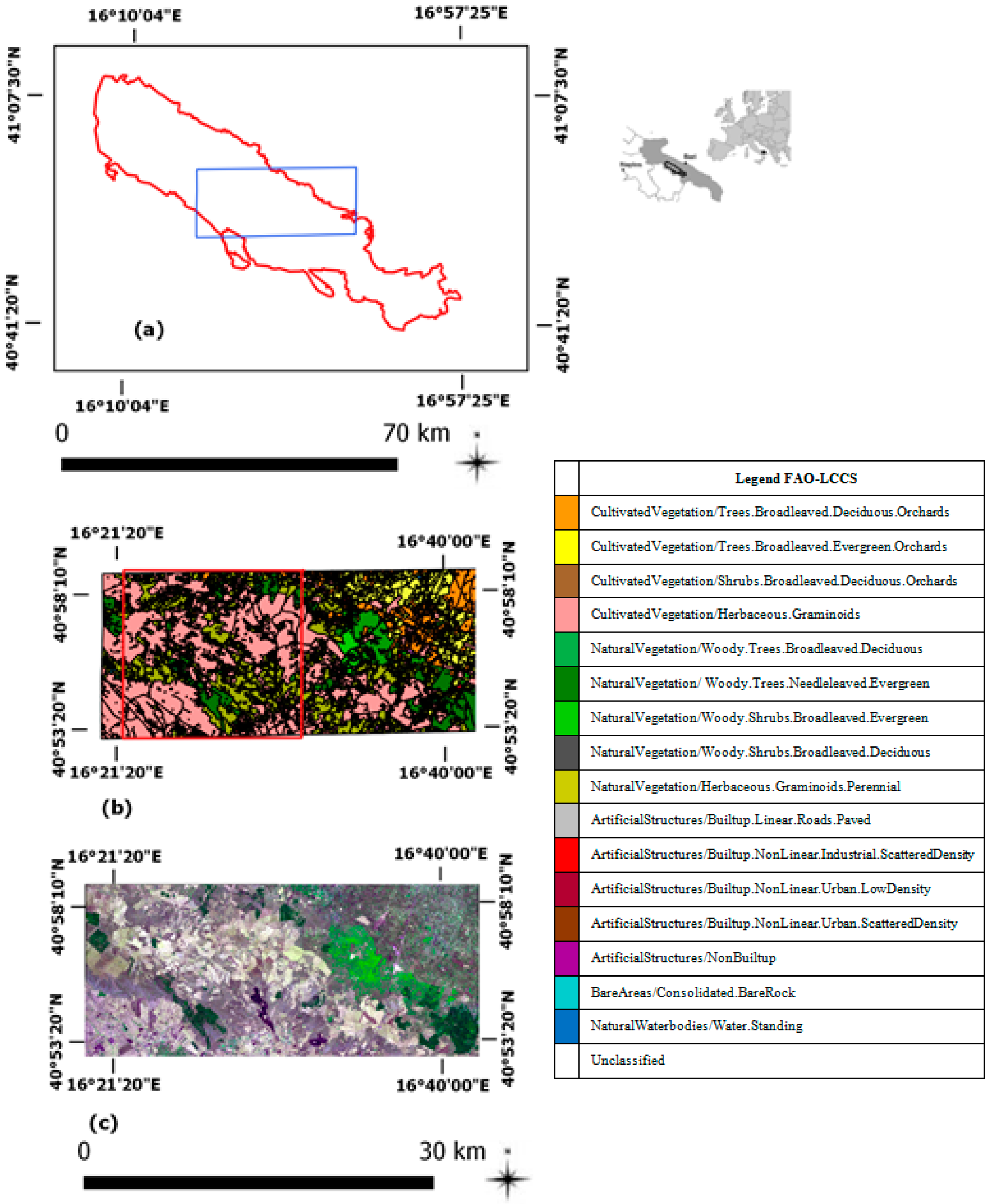
2.1.1. Italian Site
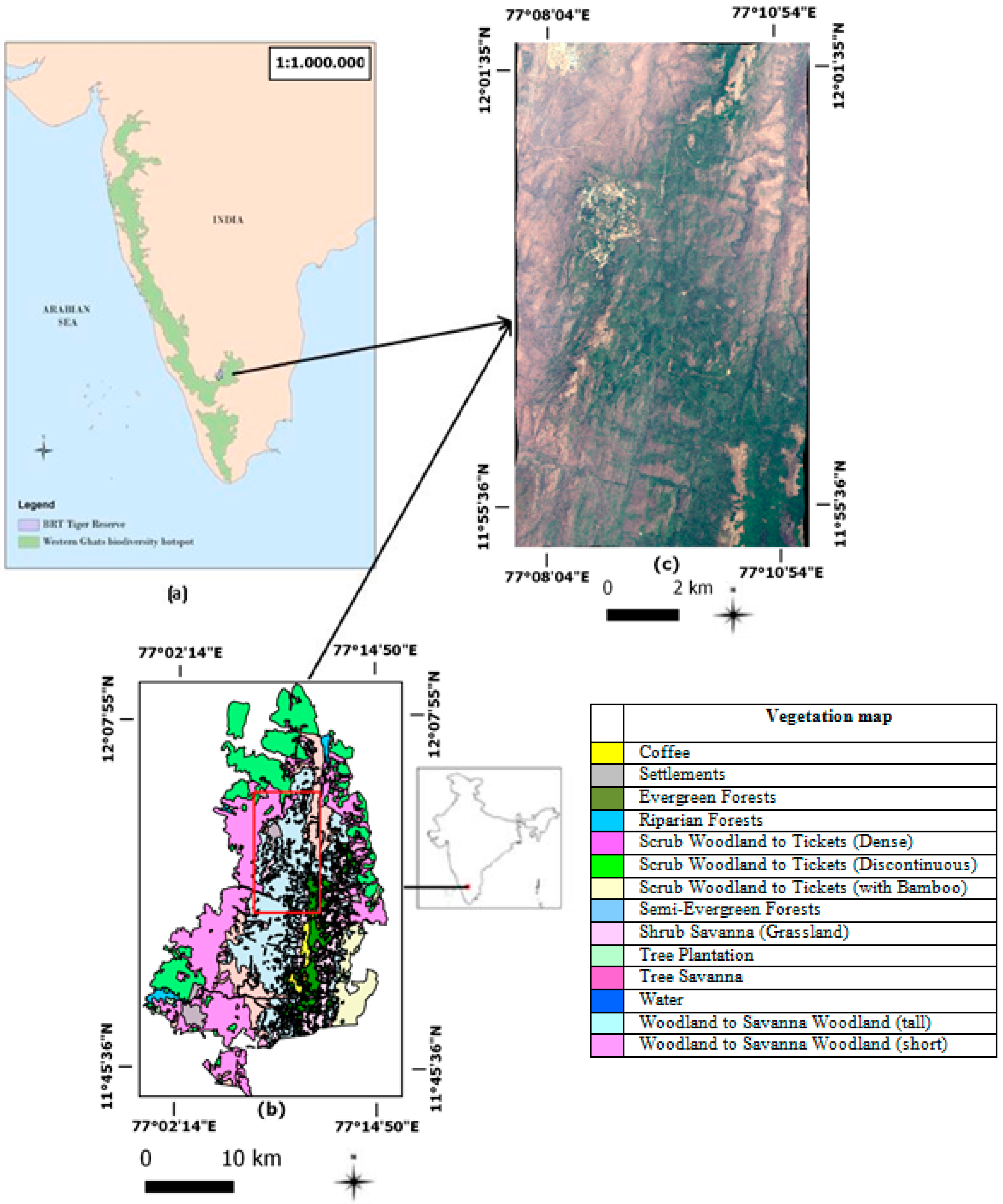
2.1.2. Indian Site
2.2. Methods
- One detected changes at HR comparing the NDVI images from the two Landsat images (Image to Image comparison) acquired at T1 and T2, with T2 > T1.
- The other detected changes at HR and VHR by Cross Correlation Analysis (Map to Image comparison).
2.3. Accuracy Assessment
3. Results
3.1. Italian Site
3.2. Indian Site
4. Discussion
4.1. The Italian site
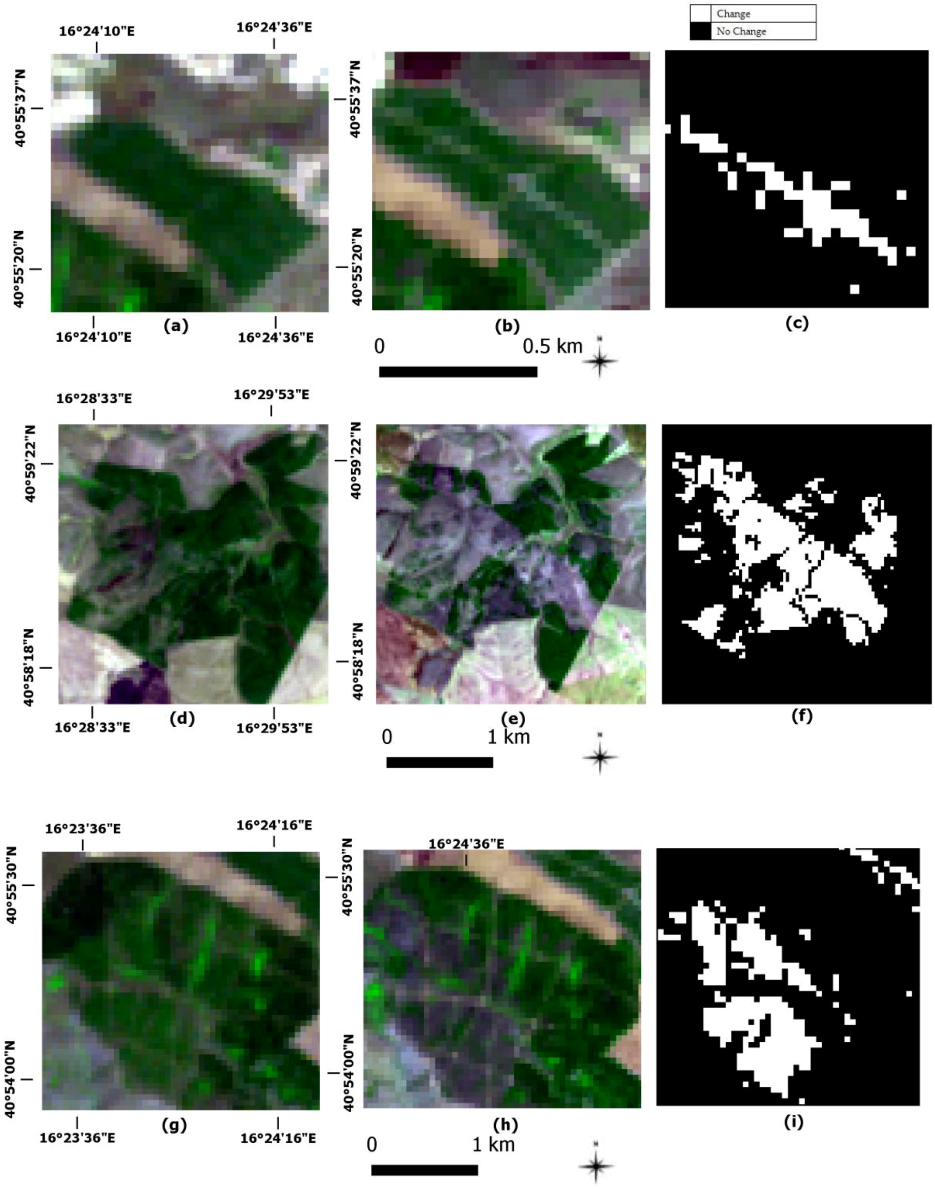
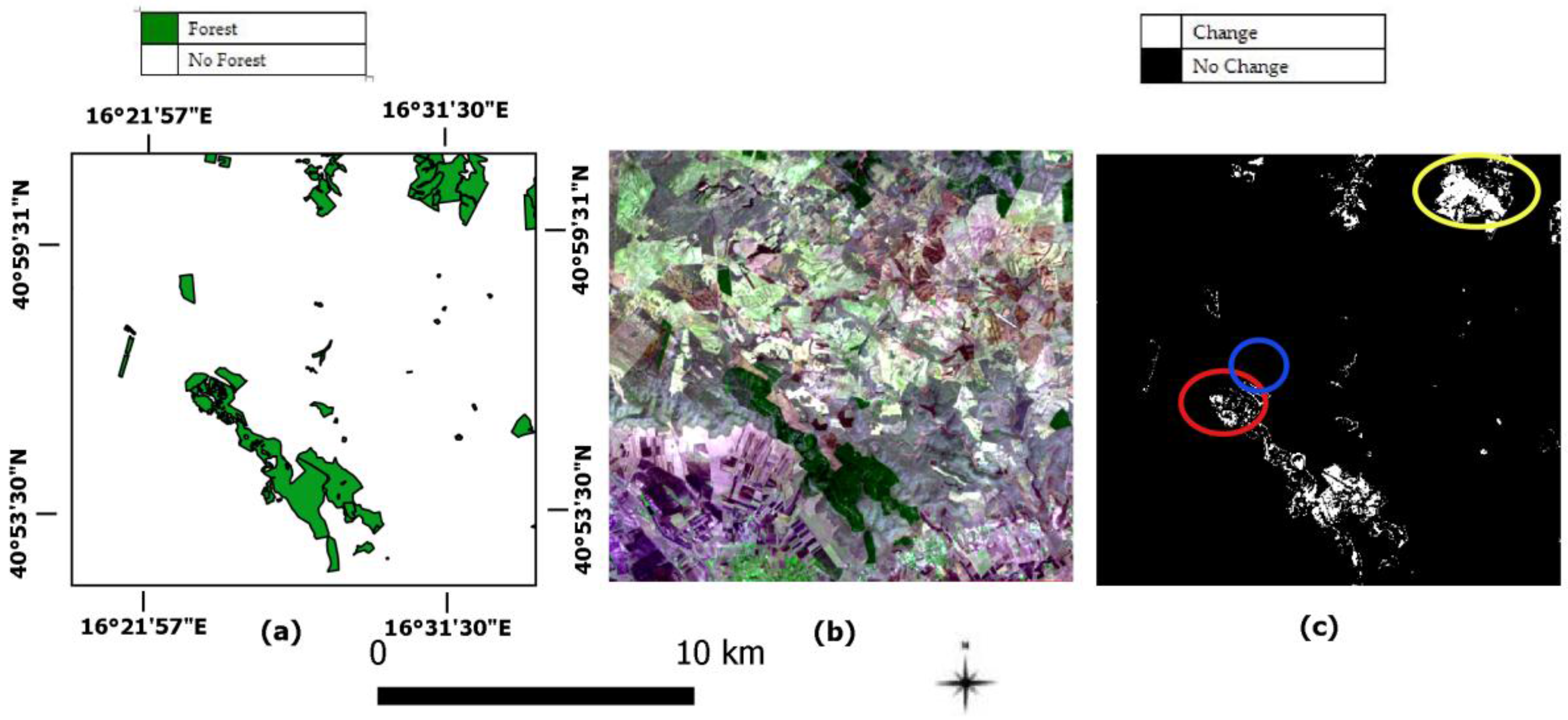
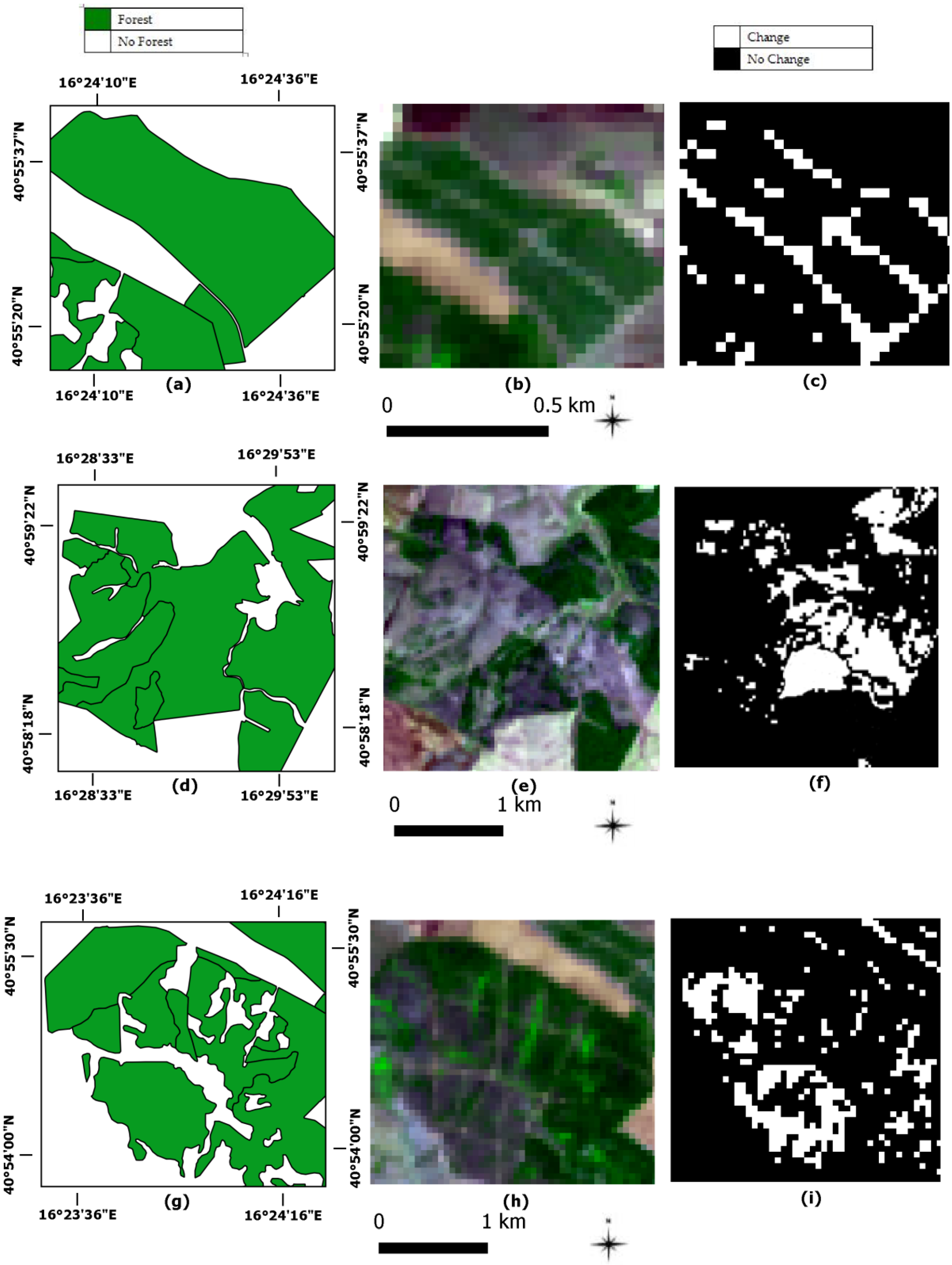
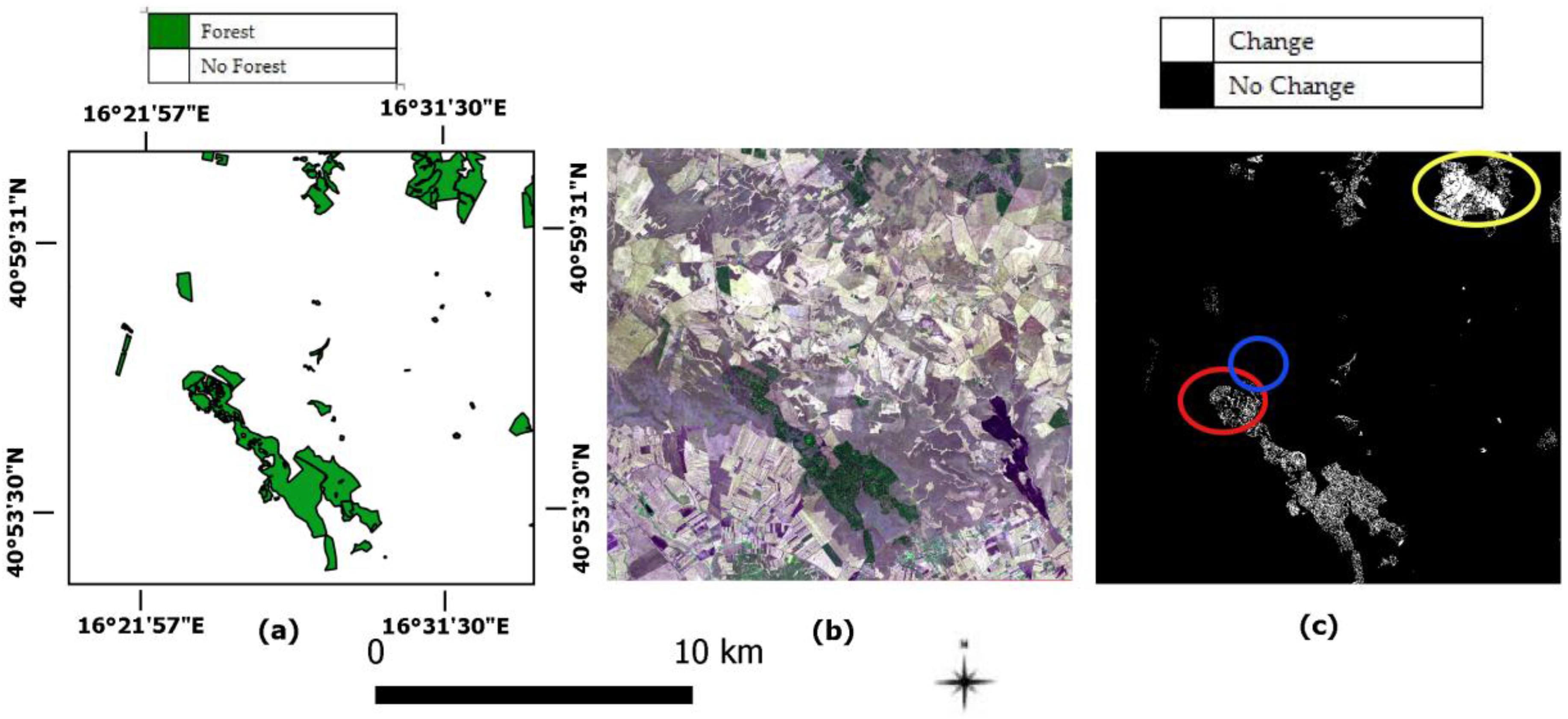
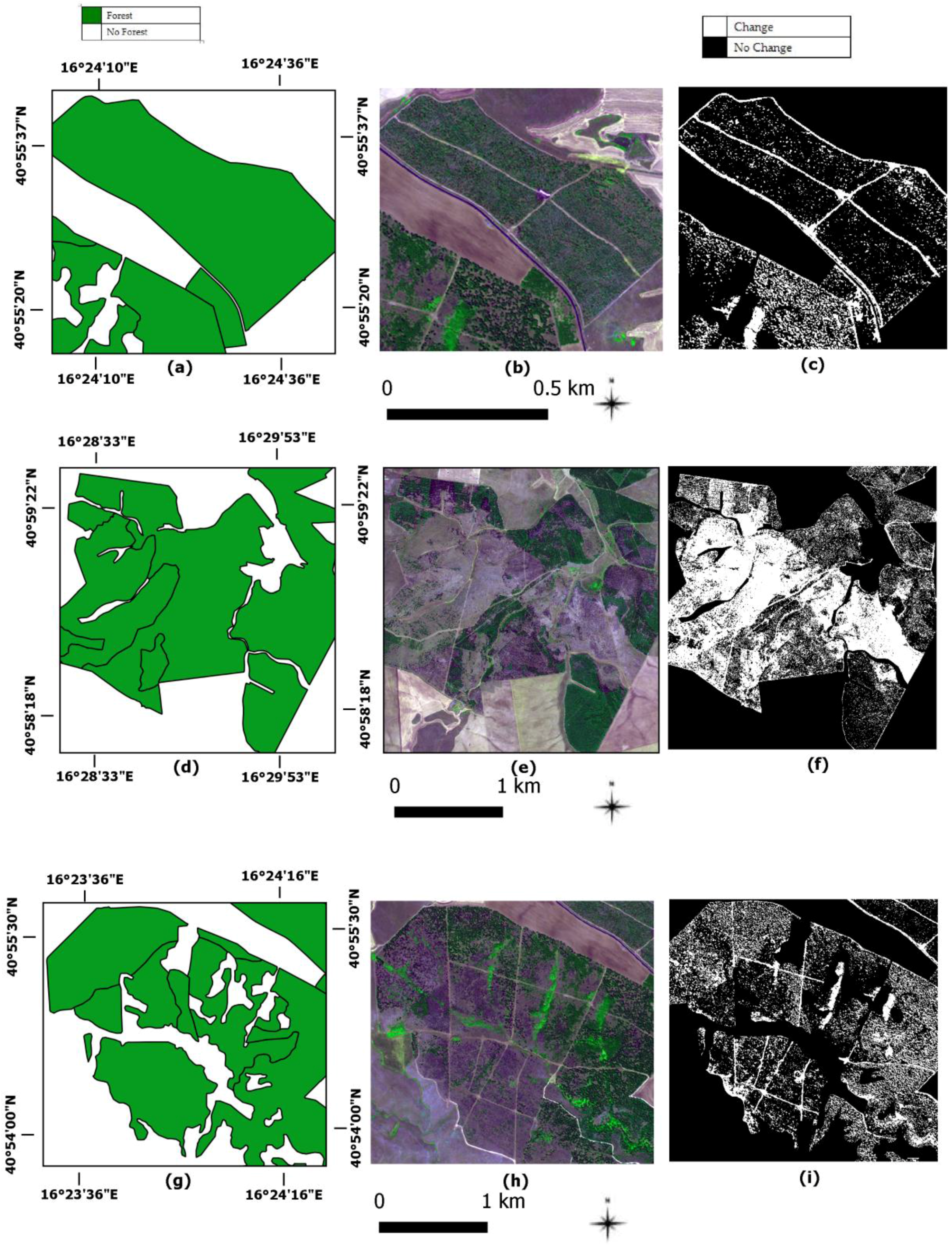
- At comparable scale (HR), when CCA_HR is adopted, the overall accuracy is larger (68.19%) than the accuracy value obtained by DIFF_NDVI_HR (52.18%) with a significant reduction of the error in the stratified changed area estimate (from ±111.71 ha to ±36.9 ha). For example, the change area that is visible in Figure 5c (CCA_HR), close to the red and blue circles, was not detected in Figure 3c (DIFF_NDVI_HR). Moreover, the close-up in Figure 6c (CCA_HR) shows detailed changes due to new roads construction within and in the borders of the forest. These changes, which are clearly visible at VHR in Figure 7b (i.e., the Worldview2 image at T2), are not detected by DIFF_NDVI_HR (Figure 4c), hence the underestimated changes in this case. In addition, CCA_HR analyses are more cost effective, since only the T2 pixels that correspond to the specific target class in T1 must be analysed. The VHR image allows validation of the changes detected when in-field campaigns may not be feasible (Figure 7b).
- At fine scale, CCA_VHR provides the best overall accuracy (71.11%). This value is very close to the CCA_HR result (68.19%) but the former value is associated with the lowest error in the stratified changed area estimation (±2.48 ha), as already demonstrated in a previous study for grasslands ecosystems [21]. Both forest fragmentation by roads and changes in forest density are confirmed at finer scale by CCA_VHR (Figure 8c). Therefore, the best change results can be achieved by comparing fine scale LC/LU map with one single VHR image. These findings appear to support arguments in favour of the acquisition and storage of VHR images on protected areas at a regular base and, possibly, at a reduced cost for those institutions in charge of the protected areas management [8].
4.2. The Indian Site
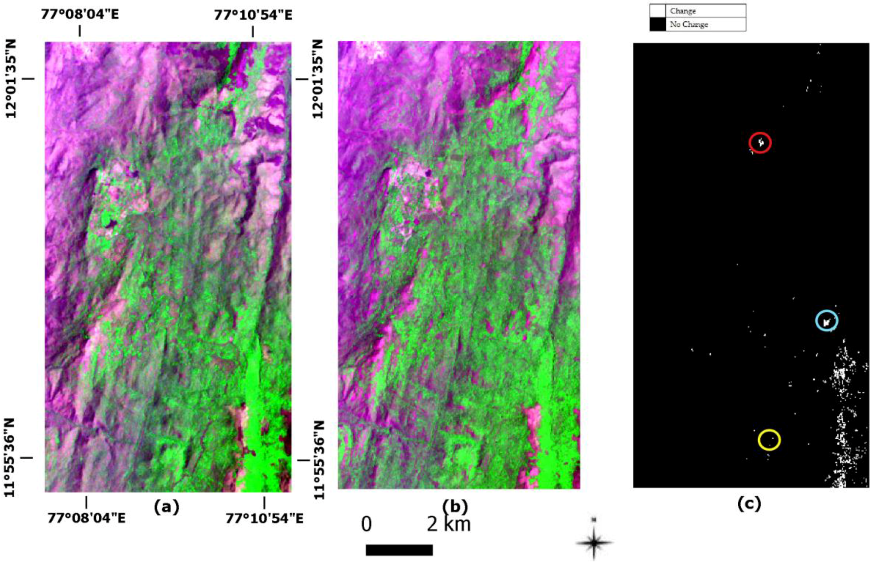
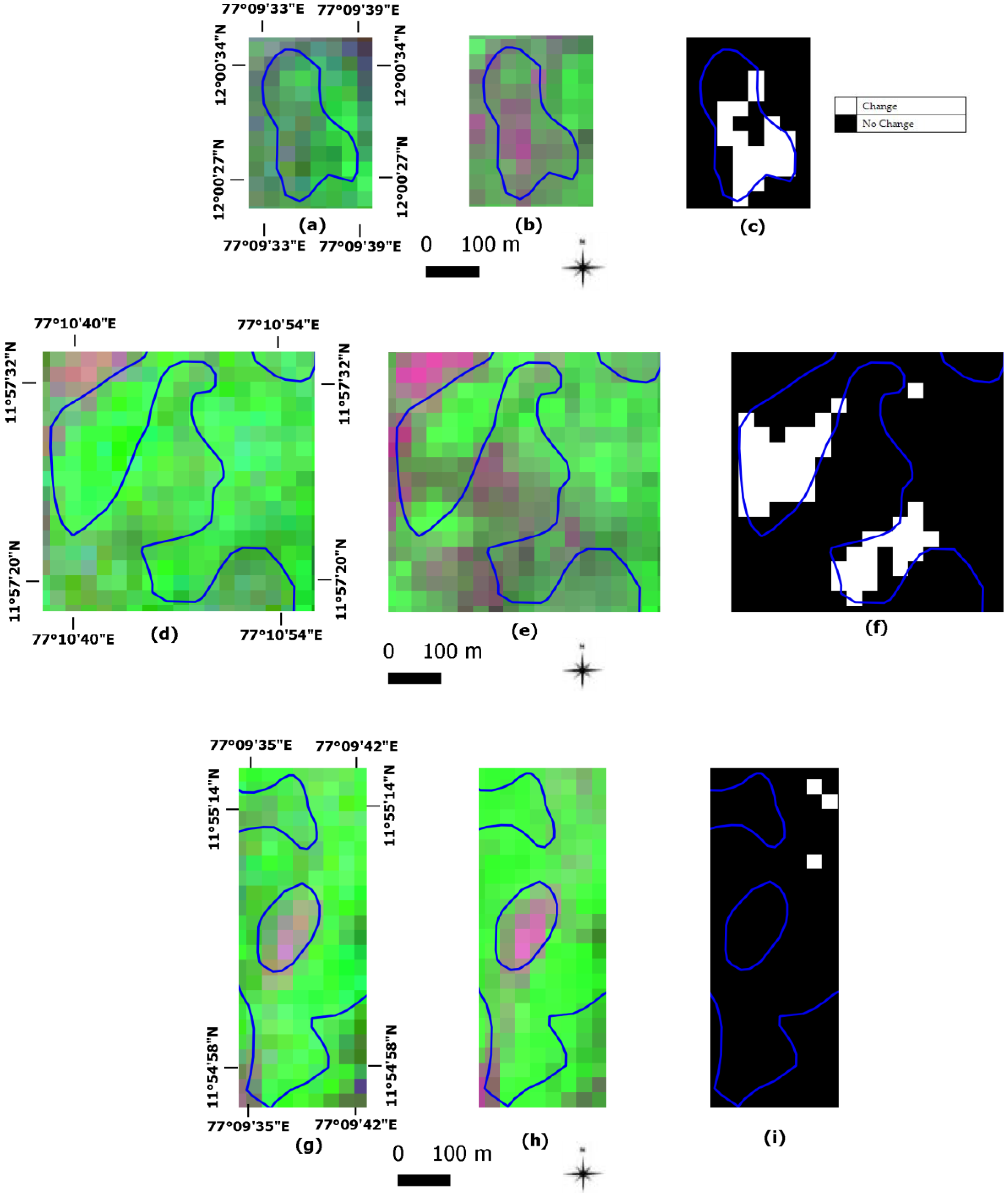
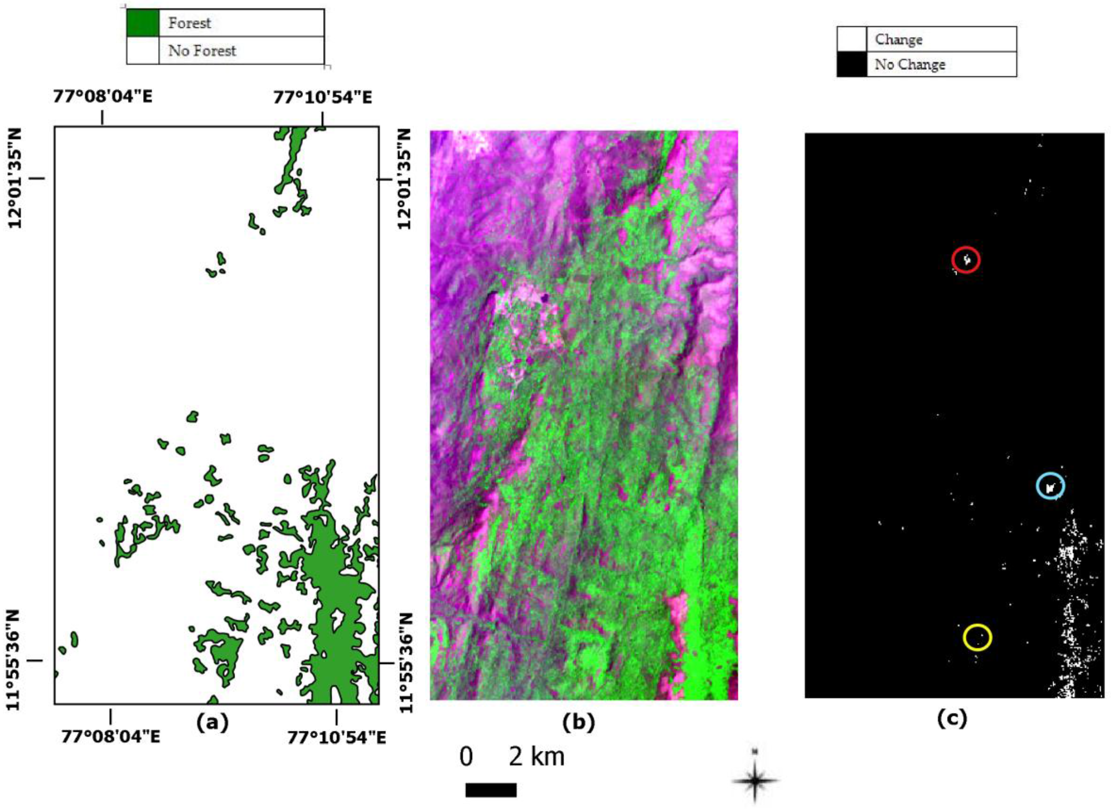
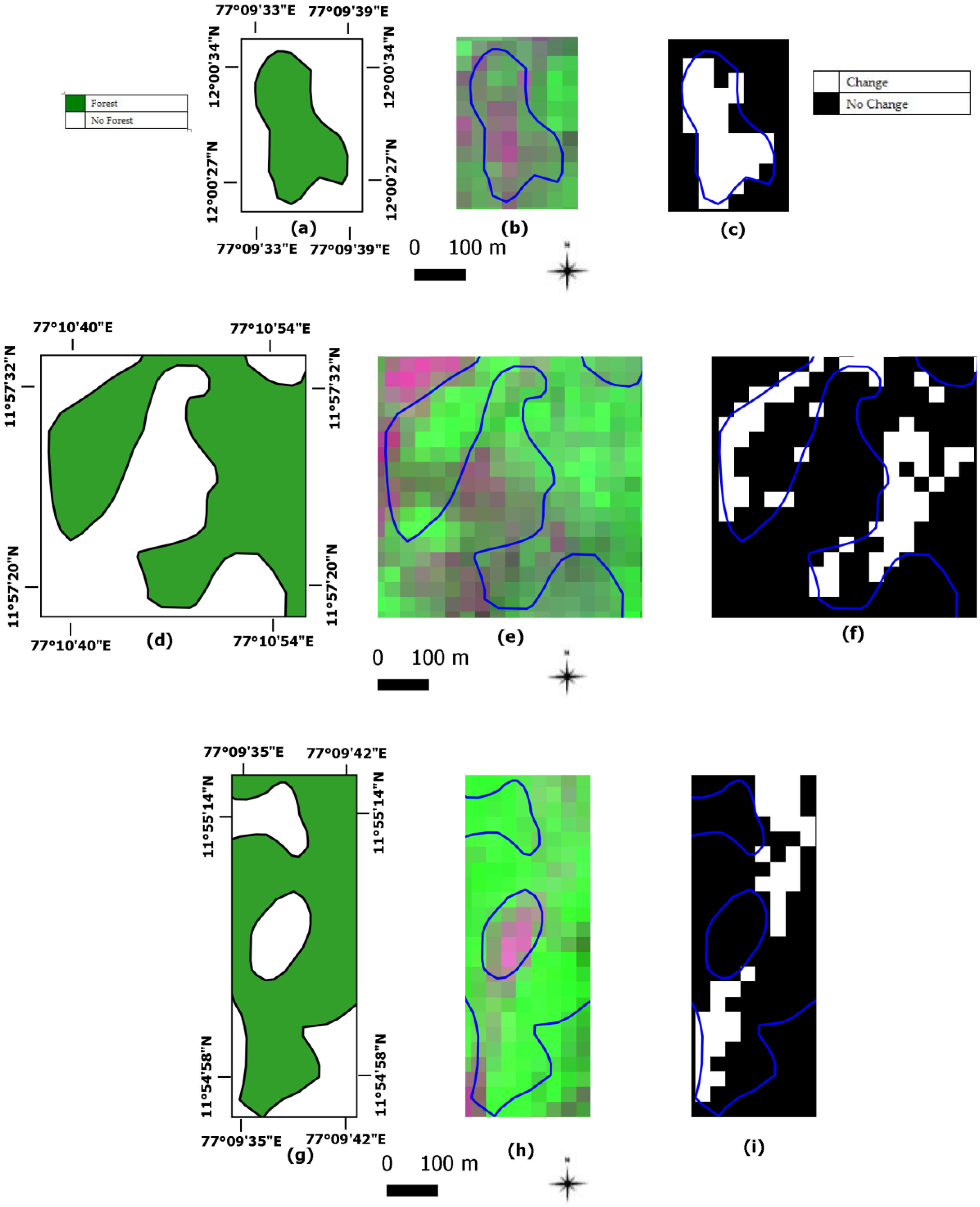
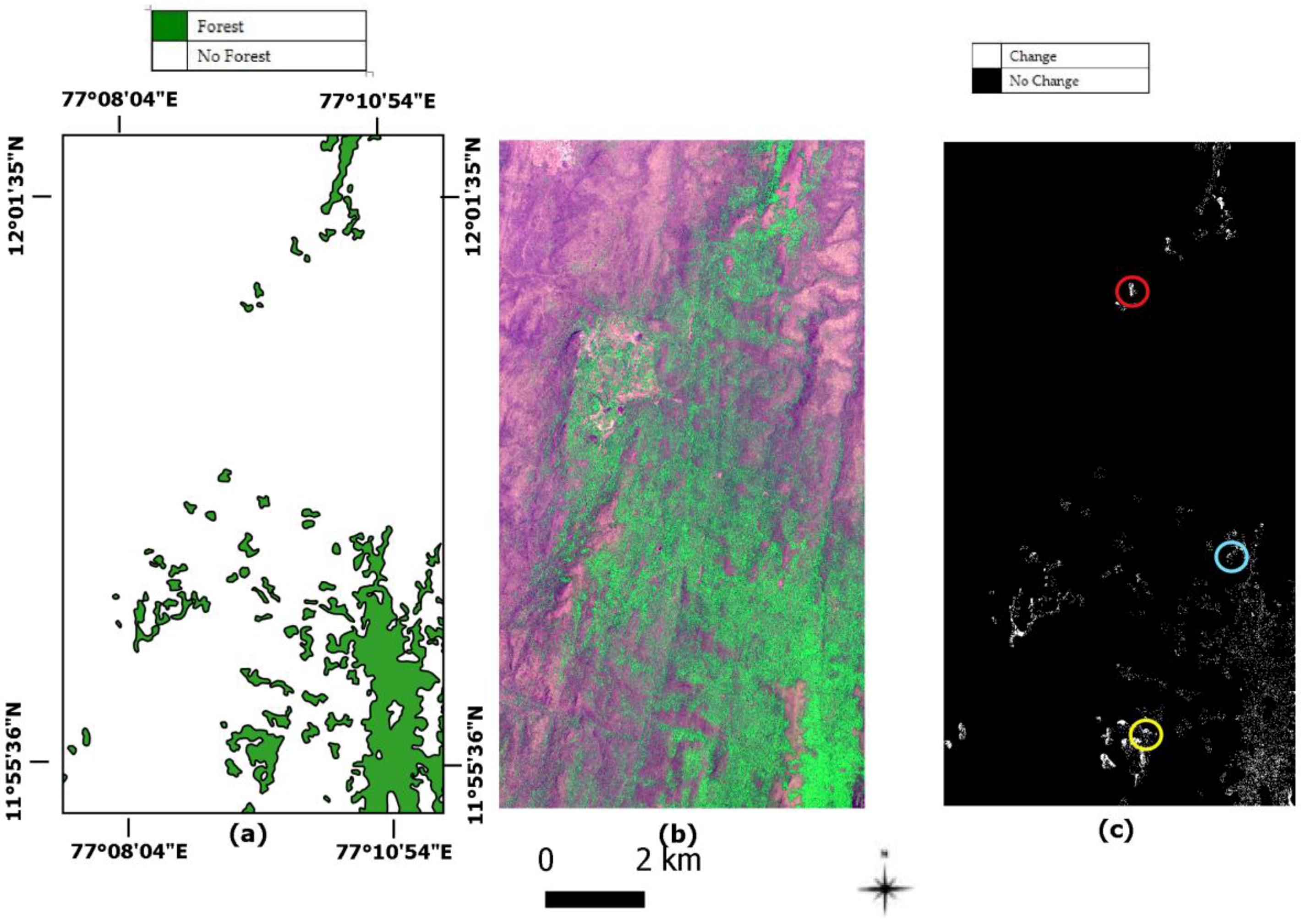
- The changes identified in the evergreen forest by the DIFF_NDVI_HR are underestimated in comparison to the ones found by CCA_HR at the same scale. For instance, Figure 12c shows changes that are completely missed in Figure 10c. In addition, in the Indian experiment, the overall accuracy of CCA_HR is larger (82.29%) than the one from the DIFF_NDVI_HR (63.33%) with comparable errors in the stratified area estimate (Table 4). At HR, the results appear to confirm the inadequacy of direct NDVI image comparison for change detection in tropical forest (Figure 10i).
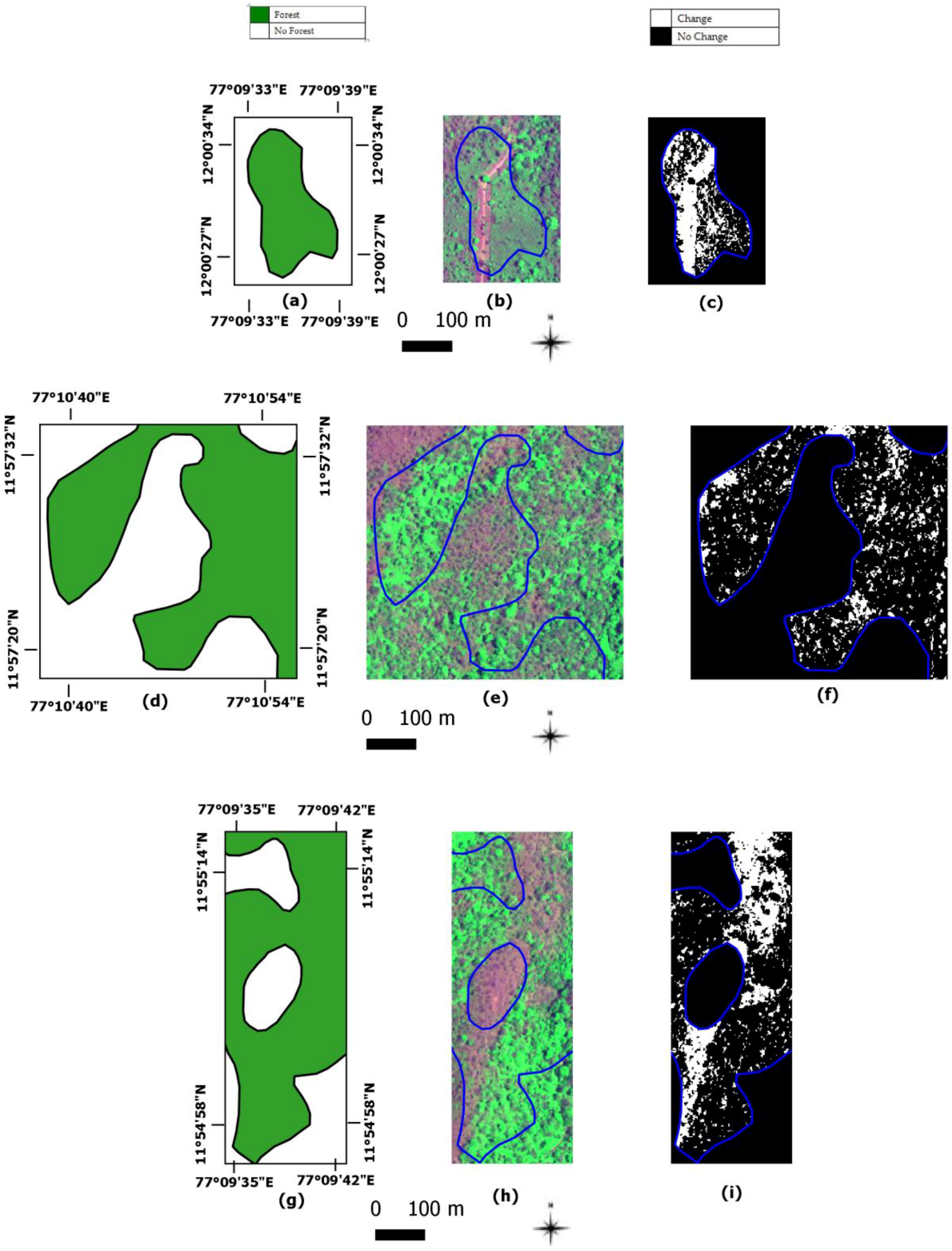
- For validation purposes, CCA was carried out also at VHR resolution, even if the scale of the existing LC/LU map is coarse (1:50,000). The output change images in the Figure 14c,f,i clearly validate the changes detected at HR by both CCA_HR. The changes observed may be mainly due to both deforestation and construction of new roads. Although the findings reported appear to be very interesting, more detailed information on the conditions of the changes in the tropical forest would be required. These may involve complementary in-field inspection and the collaboration of different scientific expertise.
- It must be recalled that, in the Indian site, the evergreen forest layer is adjacent to different vegetable classes named “woodland to savanna woodland (tall)” and “tree savanna”. Figure 10d,e evidence both such conditions and the presence of some changes in the vegetable classes which remained un-detected by CCA (Figure 10e). This discrepancy can be ascribed to the a priori class selection made to perform CCA analysis. In order to have inclusive detection of overall changes, additional CCA processing steps should be applied. However, the more inclusive process would be time consuming. On the other hand, DIFF_NDVI_HR can yield more comprehensive detection of possible changes in one single processing step, but the resulting overall accuracy would be lower than the one obtained through CCA. Undoubtedly, the choice of the most appropriate change detection technique will depend on specific user’s requirements as well as comprehensive cost effectiveness.
5. Conclusions
Acknowledgments
Author Contributions
Conflicts of Interest
References
- Nativi, S.; Mazzetti, P.; Geller, G.N. Environmental model access and interoperability: The GEO model web. Environ. Model. Softw. 2013, 39, 214–228. [Google Scholar] [CrossRef]
- Pettorelli, N.; Laurance, B.; O’Brien, T.; Wegmann, M.; Nagendra, H.; Turner, W. Satellite remote sensing for applied ecologists: Opportunities and challenges. J. Appl. Ecol. 2014, 51, 839–848. [Google Scholar] [CrossRef]
- Turner, W.; Rondinini, C.; Pettorelli, N.; Mora, B.; Leidner, A.K.; Szantoi, Z.; Buchanana, G.; Dech, S.; Dwyer, J.; Herold, M.; et al. Free and open-access satellite data are key to biodiversity conservation. Biol. Conserv. 2015, 182, 173–176. [Google Scholar] [CrossRef]
- Nagendra, H.; Lucas, R.; Honrado, J.P.; Jongman, R.; Tarantino, C.; Adamo, M.; Mairota, P. Remote sensing for conservation monitoring: Assessing protected areas, habitat extent, habitat condition, species diversity, and threats. Ecol. Indic. 2013, 33, 45–59. [Google Scholar] [CrossRef]
- Nagendra, H.; Mairota, P.; Marangi, C.; Lucas, R.; Dimopoulos, P.; Honrado, J.P.; Niphadkar, M.; Mücher, C.A.; Tomaselli, V.; Panitsa, M.; et al. Satellite Earth observation data to identify anthropogenic pressures in selected protected areas. Intern. J. Appl. Earth Observ. Geoinf. 2015, 37, 124–132. [Google Scholar] [CrossRef]
- Blonda, P.; Lucas, R.M.; Honrado, J.P. From Space to species: Solutions for biodiversity monitoring. Window GMES Success Stories 2012, 66–73. [Google Scholar]
- Blonda, P.; Jongman, R.; Stutte, J.; Dimopoulos, P. From Space to species. Safeguarding biodiversity in Europe. Intern. Innov. Environ. 2012, 86–88. [Google Scholar]
- Kennedy, R.E.; Andrefouet, S.; Cohen, W.B. Bringing an ecological view of change to Landsat-based remote sensing. Front. Ecol. Environ. 2014, 12, 339–346. [Google Scholar] [CrossRef] [Green Version]
- Sorrano, P.A.; Cheruvelil, K.S.; Bissel, E.G.; Bremigan, M.T.; Downing, J.A.; Fergus, C.E.; Filstrup, C.T.; Henry, E.N.; Lottig, N.R.; Stanley, E.H.; et al. Cross-scale interactions: Quantifying multi-scaled cause–effect relationships in macrosystems. Front. Ecol. Environ. 2014, 12, 65–73. [Google Scholar] [CrossRef]
- Bruzzone, L.; Bovolo, F. A novel framework for the design of change-detection systems for Very-High-Resolution remote sensing images. Proc. IEEE 2013, 101, 609–630. [Google Scholar] [CrossRef]
- Bovolo, F.; Marchesi, S.; Bruzzone, L. A framework for automatic and unsupervised detection of multiple changes in multitemporal images. IEEE Trans. Geosci. Remote Sens. 2012, 50, 2196–2212. [Google Scholar] [CrossRef]
- Tarantino, C.; Blonda, P.; Pasquariello, G. Remote sensed data for automatic detection of land use changes due to human activity in support to landslide studies. Nat. Hazards 2007, 4, 245–267. [Google Scholar] [CrossRef]
- Chen, G.; Hay, G.J.; Carvalho, L.M.T.; Wulder, M.A. Object-based change detection. Intern. J. Remote Sens. 2012, 33, 4434–4457. [Google Scholar] [CrossRef]
- Foody, G.M. Ground reference data error and the mis-estimation of the area of landcover change as a function of its abundance. Remote Sens. Lett. 2013, 4, 783–792. [Google Scholar] [CrossRef]
- Olofsson, P.; Foody, G.M.; Stehman, S.V.; Woodcock, C.E. Making better use of accuracy data in land change studies: Estimating accuracy and area and quantifying uncertainty using stratified estimation. Remote Sens. Environ. 2013, 129, 122–131. [Google Scholar] [CrossRef]
- Fuller, R.M.; Smith, G.M.; Devereux, B.J. The characterization and measurement of land cover change through remote sensing: Problems in operational applications? Int. J. Appl. Earth Observ. Geoinf. 2003, 4, 243–253. [Google Scholar] [CrossRef]
- Hall, O.; Hay, G. A Multiscale object-specific approach to digital change detection. Intern. J. Appl. Earth Observ. Geoinf. 2003, 4, 311–327. [Google Scholar] [CrossRef]
- Lucas, R.; Blonda, P.; Bunting, P.; Jones, G.; Inglada, J.; Arias, M.; Kosmidou, V.; Petrou, Z.I.; Manakos, I.; Adamo, M.; et al. The Earth Observation Data for Habitat Monitoring (EODHaM) system. Intern. J. Appl. Earth Observ. Geoinf. 2015, 37, 17–28. [Google Scholar] [CrossRef] [Green Version]
- Koeln, G.; Bissonnette, J. Cross-Correlation Analysis: Mapping landcover changes with a historic landcover database and a recent, single-date, multispectral image. In Proceedings of the 2000 ASPRS Annual Convention, Washington, DC, USA, 22–26 May 2000.
- Comparison of Land Use and Land Cover Change Detection Methods. Available online: https://www.researchgate.net/publication/228543190_A_comparison_of_land_use_and_land_cover_change_detection_methods (accessed on 12 April 2002).
- Tarantino, C.; Adamo, M.; Lucas, R.; Blonda, P. Detection of changes in semi-natural grasslands by cross correlation analysis with WorldView-2 images and new Landsat 8 data. Remote Sens. Environ. 2016, 175, 65–72. [Google Scholar] [CrossRef]
- Olofsson, P.; Foody, G.M.; Herold, M.; Stehman, S.V.; Woodcock, C.E.; Wulder, M.A. Good practices for estimating area and assessing accuracy of land change. Remote Sens. Environ. 2014, 148, 42–57. [Google Scholar] [CrossRef]
- Mairota, P.; Cafarelli, B.; Boccaccio, L.; Leronni, V.; Labadessa, R.; Kosmidou, V. Using landscape structure to develop quantitative baselines for protected area monitoring. Ecol. Indic. 2013, 33, 82–95. [Google Scholar] [CrossRef]
- Tomaselli, V.; Dimopoulos, P.; Marangi, C.; Kallimanis, A.S.; Adamo, M.; Tarantino, C.; Panitsa, M.; Terzi, M.; Veronico, G.; Lovergine, F.; et al. Translating land cover/land use classifications to habitat taxonomies for landscape monitoring: A mediterranean assessment. Landsc. Ecol. 2013, 28, 905–930. [Google Scholar] [CrossRef]
- BIO_SOS Project Website. Available online: www.biosos.eu (accessed on 11 December 2010).
- US Geological Survey Website. Available online: http://earthexplorer.usgs.gov/ (accessed on 18 July 2016).
- Irons, J.R.; Dwyer, J.L.; Barsi, J.A. The next Landsat satellite: The Landsat data continuity mission. Remote Sens. Environ. 2012, 122, 11–21. [Google Scholar] [CrossRef]
- Hall, F.G.; Strebel, D.E.; Nickeson, J.E.; Goetz, S.G. Radiometric rectification: Toward a common radiometric response among multidate, multisensor images. Remote Sens. Environ. 1991, 35, 11–27. [Google Scholar] [CrossRef]
- Congalton, R.G.; Kass, G. Assessing the Accuracy of Remotely Sensed Data: Principle and Practices, 2nd ed.; CRC Press/Taylor & Francis Group: Boca Raton, FL, USA, 2009. [Google Scholar]
- WAVES–World Bank Group. Natural Capital Accounting: Forests. 2016. Available online: https://www.wavespartnership.org/sites/waves/files/kc/NCA-Forest%20Accounts.pdf (accessed on 13 May 2016).
- Food and Agriculture Organization (FAO). State of the World’s Forests. 2016. Available online: http://www.fao.org/3/a-i5588e.pdf (accessed on 18 July 2016).
- United Nations (UN). Sustainable Development Goals. 2016. Available online: https://sustainabledevelopment.un.org (accessed on 18 July 2016).


| Experiment | Input Data at T1 | Time T2 | Change Method | Change Method Acronym |
|---|---|---|---|---|
| 1 | Landsat 7 ETM image: 27 July 2006 | Landsat 8 OLS image: 7 August 2013 | NDVI direct comparison by image differencing | DIFF_NDVI_HR |
| 2.a | Forest layer from existing Land Cover/Land Use Map dated 2006 | Landsat 8 OLS image: 7 August 2013 | Cross Correlation Analysis | CCA_HR |
| 2.b | Worldview-2 image: 6 July 2012 | CCA_VHR |
| Experiment | Input Data at T1 | Time T2 | Change Method | Change Method Acronym |
|---|---|---|---|---|
| 1 | Landsat 5 image: 16 March 1997 | Landsat 8 OLS image: 20 March 2016 | NDVI direct comparison by image differencing | DIFF_NDVI_HR |
| 2.a | Tropical evergreen forest target class of interest from existing LC/LU map dated 1998 | Landsat 8 OLS image: 20 March 2016 | Cross Correlation Analysis | CCA_HR |
| 2.b | Worldview-2 image: 14 March 2013 | CCA_VHR |
| Change: Transition from Forest to No Forest—at Different TH for an Area of 1518 ha (at T1) | |||||||||
|---|---|---|---|---|---|---|---|---|---|
| Experiment | Method | TH | Change User’s Acc.% | Change Producer’s Acc.% | No Change User’s Acc.% | No Change Producer’s Acc.% | Overall Acc.% | Am (ha) Mapped Area of Change | Stratified Changed Area Estimate with 95% Conf. Interv. (ha) |
| 1 | DIFF_NDVI_HR | DIFF > 0 | 83.58 ± 1.50 | 10.87 ± 0.57 | 49.88 ± 1.09 | 97.65 ± 0.50 | 52.18 ± 1.02 | 371.61 | 2856.19 ± 111.71 |
| 2.a | CCA_HR | CCA > μ + 1σ | 72.96 ± 0.07 | 94.77 ± 0.01 | 46.49 ± 0.64 | 11.45 ± 0.05 | 71.11 ± 0.08 | 1412.13 | 1087.13 ± 2.48 |
| CCA > μ + 2σ | 74.92 ± 0.08 | 75.33 ± 0.03 | 42.90 ± 0.23 | 42.35 ± 0.13 | 65.30 ± 0.09 | 1062.07 | 1056.19 ± 2.64 | ||
| CCA > μ + 3σ | 82.27 ± 0.08 | 48.01 ± 0.05 | 41.12 ± 0.13 | 77.83 ± 0.13 | 57.50 ± 0.08 | 604.07 | 1035.24 ± 2.51 | ||
| 2.b | CCA_VHR | CCA > μ + 1σ | 69.44 ± 1.05 | 92.28 ± 0.15 | 59.42 ± 5.95 | 21.78 ± 0.98 | 68.19 ± 1.18 | 1364.31 | 1026.71 ± 36.94 |
| CCA > μ + 2σ | 70.51 ± 1.07 | 74.63 ± 0.41 | 52.51 ± 3.74 | 47.34 ± 1.78 | 64.47 ± 1.44 | 1036.44 | 979.30 ± 45.03 | ||
| CCA > μ + 3σ | 72.97 ± 1.14 | 49.25 ± 0.73 | 45.66 ± 2.27 | 70.05 ± 2.09 | 57.12 ± 1.40 | 654.21 | 969.44 ± 43.69 | ||
| Change: Transition from Evergreen Forest to No Evergreen Forest—at Different TH for an Area of 911 ha (at T1) | |||||||||
|---|---|---|---|---|---|---|---|---|---|
| Experiment | Method | TH | Change User’s Acc.% | Change Producer’s Acc.% | No Change User’s Acc.% | No Change Producer’s Acc.% | Overall Acc.% | Am (ha) Mapped Area of Change | Stratified Changed Area Estimate with 95% Conf. Interv. (ha) |
| 1 | DIFF_NDVI_HR | DIFF > 0 | 44.29 ± 5.98 | 9.68 ± 1.88 | 65.26 ± 2.09 | 93.31 ± 0.62 | 63.33 ± 1.98 | 72.99 | 334.08 ± 37.31 |
| 2.b | CCA_HR | CCA > μ + 1σ | 92.03 ± 2.31 | 34.62 ± 1.78 | 81.24 ± 1.84 | 98.95 ± 0.67 | 82.29 ± 1.67 | 93.24 | 247.86 ± 32.01 |
| CCA > μ + 2σ | 98.70 ± 1.30 | 11.59 ± 0.76 | 73.54 ± 1.95 | 99.94 ± 0.16 | 74.40 ± 1.88 | 32.49 | 276.65 ± 36.02 | ||
| CCA > μ + 3σ | 100.0 ± 0.01 | 4.66 ± 0.29 | 68.91 ± 1.98 | 100.0 ± 0.01 | 69.37 ± 1.95 | 14.31 | 307.36 ± 37.24 | ||
| 2.a | CCA_VHR | CCA > μ + 1σ | 69.96 ± 0.26 | 43.96 ± 0.19 | 84.56 ± 0.16 | 94.20 ± 0.14 | 82.40 ± 0.14 | 134.53 | 214.10 ± 2.55 |
| CCA > μ + 2σ | 85.35 ± 0.33 | 10.95 ± 0.13 | 72.60 ± 0.17 | 99.21 ± 0.04 | 73.09 ± 0.16 | 34.60 | 296.76 ± 2.93 | ||
| CCA > μ + 3σ | 95.93 ± 0.30 | 2.54 ± 0.05 | 67.80 ± 0.17 | 99.95 ± 0.01 | 68.04 ± 0.17 | 7.90 | 298.53 ± 3.01 | ||
© 2016 by the authors; licensee MDPI, Basel, Switzerland. This article is an open access article distributed under the terms and conditions of the Creative Commons Attribution (CC-BY) license (http://creativecommons.org/licenses/by/4.0/).
Share and Cite
Tarantino, C.; Lovergine, F.; Niphadkar, M.; Lucas, R.; Nativi, S.; Blonda, P. Towards Operational Detection of Forest Ecosystem Changes in Protected Areas. Remote Sens. 2016, 8, 850. https://doi.org/10.3390/rs8100850
Tarantino C, Lovergine F, Niphadkar M, Lucas R, Nativi S, Blonda P. Towards Operational Detection of Forest Ecosystem Changes in Protected Areas. Remote Sensing. 2016; 8(10):850. https://doi.org/10.3390/rs8100850
Chicago/Turabian StyleTarantino, Cristina, Francesco Lovergine, Madhura Niphadkar, Richard Lucas, Stefano Nativi, and Palma Blonda. 2016. "Towards Operational Detection of Forest Ecosystem Changes in Protected Areas" Remote Sensing 8, no. 10: 850. https://doi.org/10.3390/rs8100850