
A Comparison between Drifter and X-Band Wave Radar for Sea Surface Current Estimation

 , , ,
, , ,  , and
, and
Abstract
:
1. Introduction
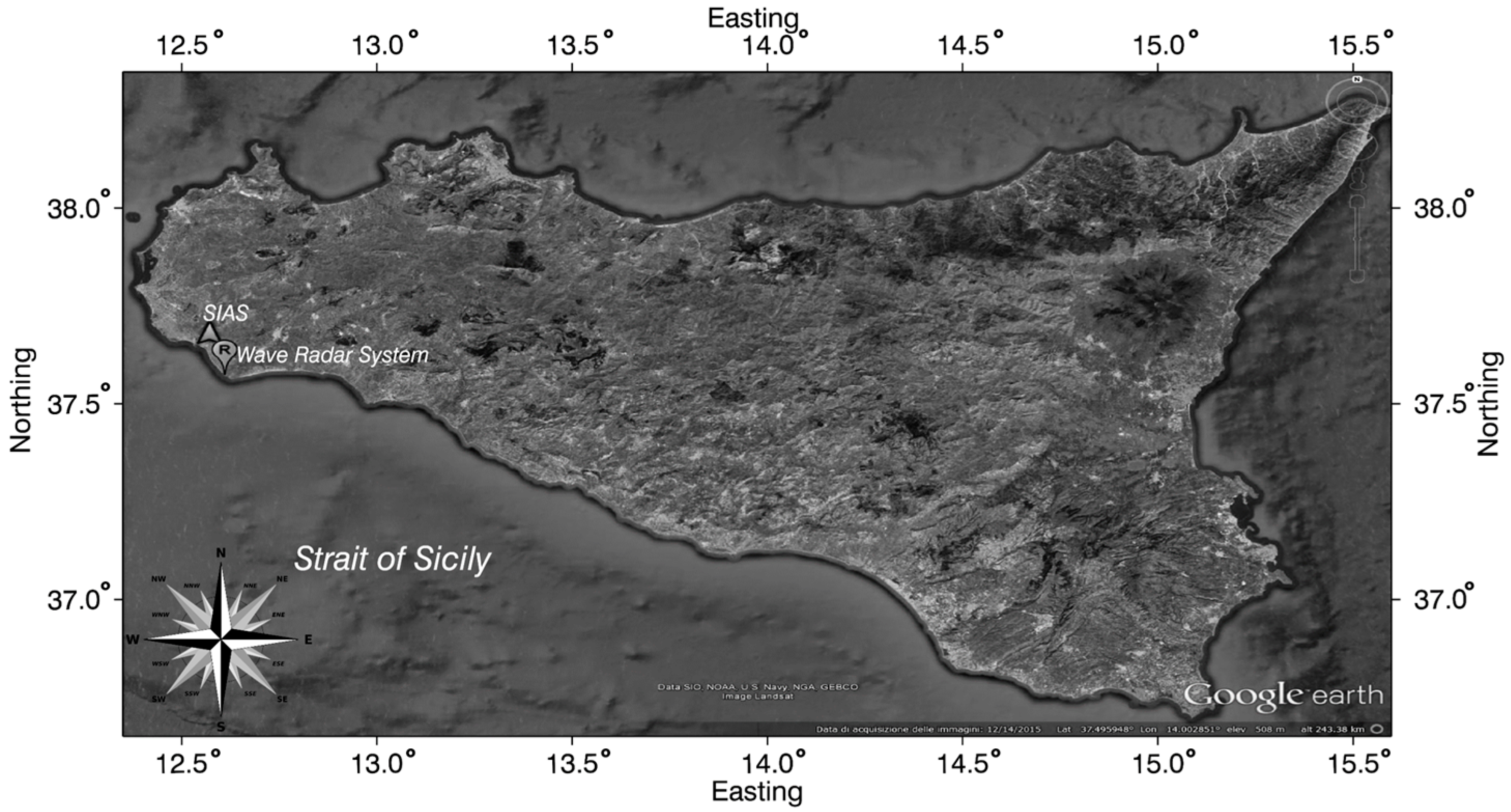
2. Test Site, Instrumentation and Methodologies
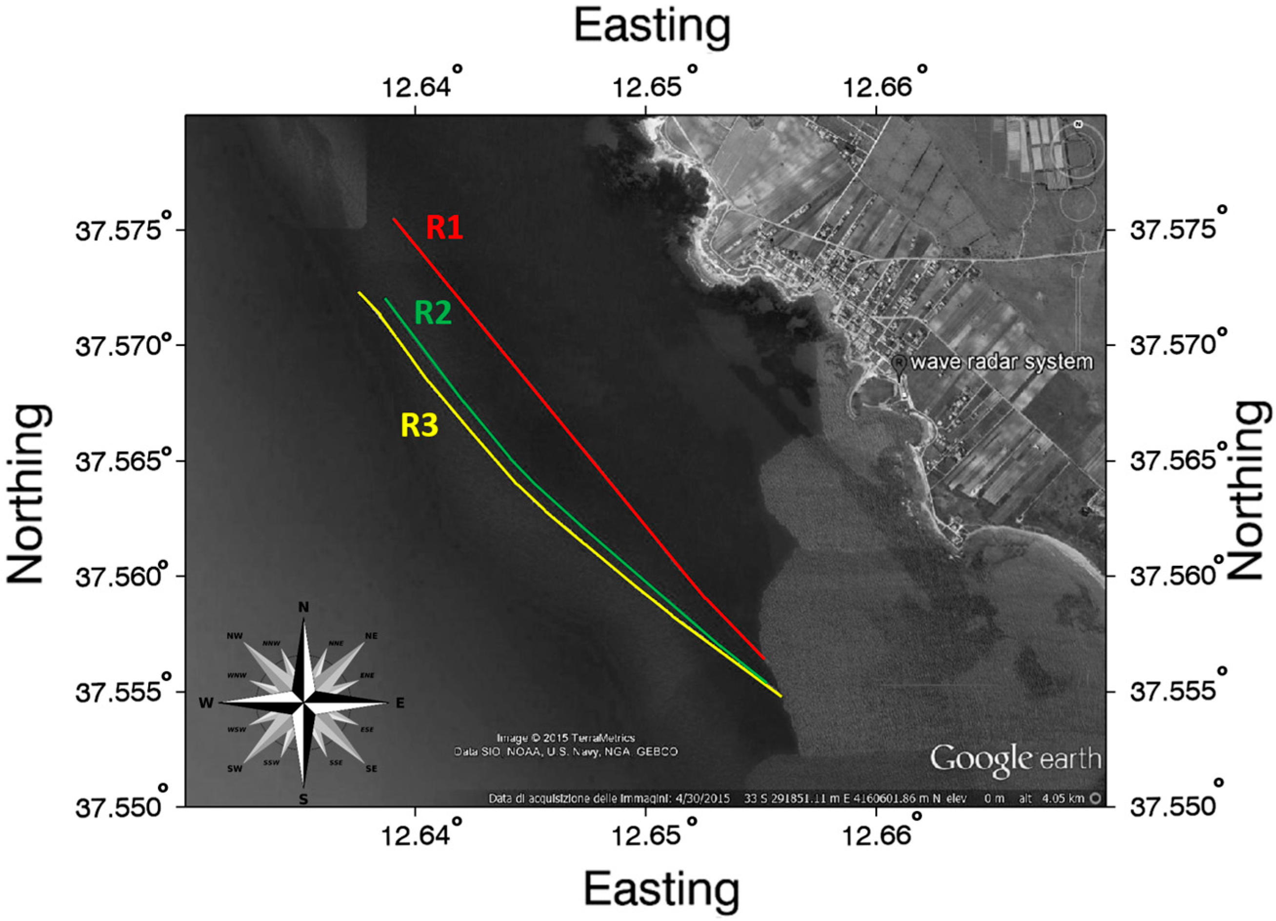
2.1. Drifters
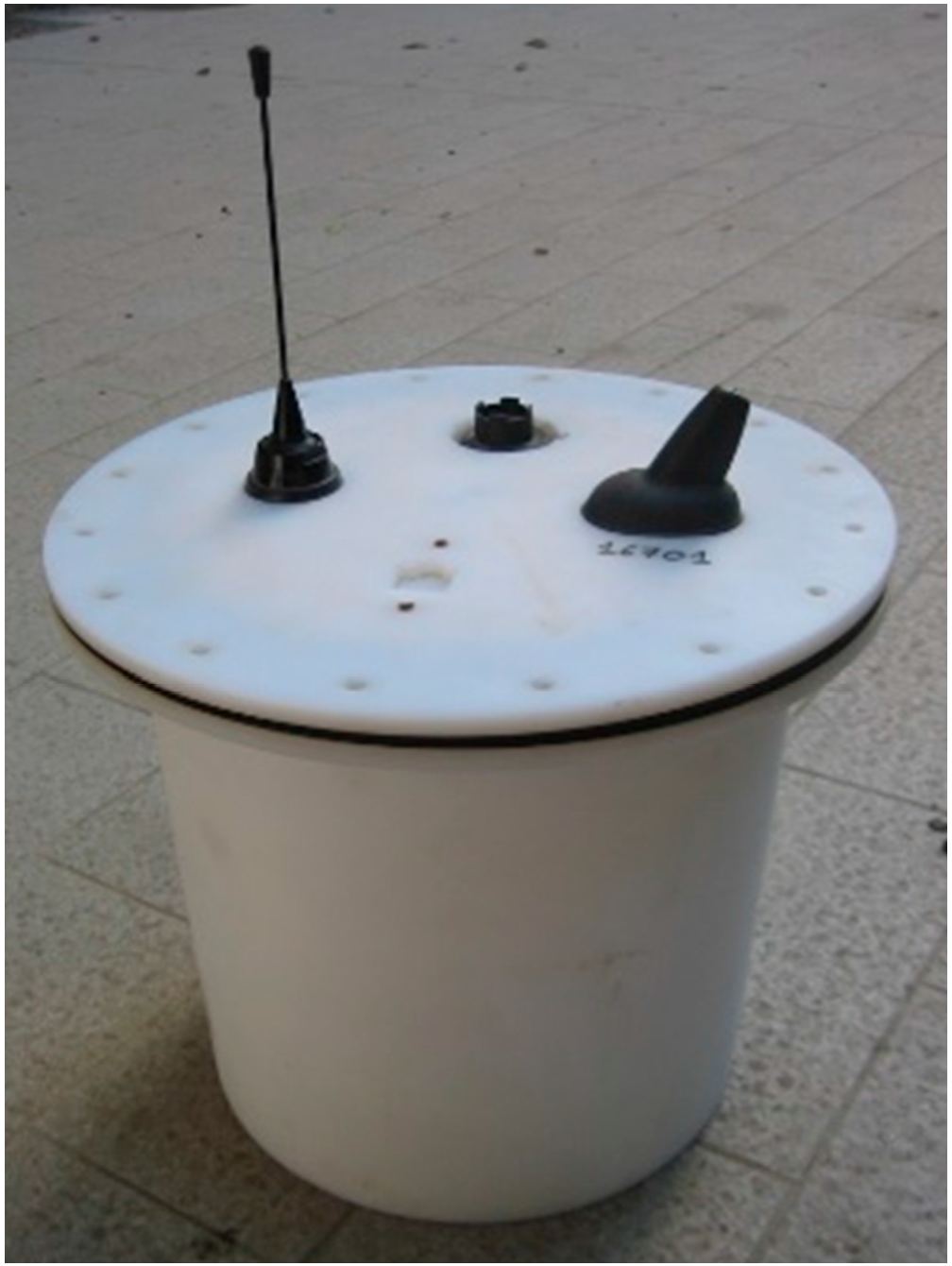
2.2. Wave Radar System
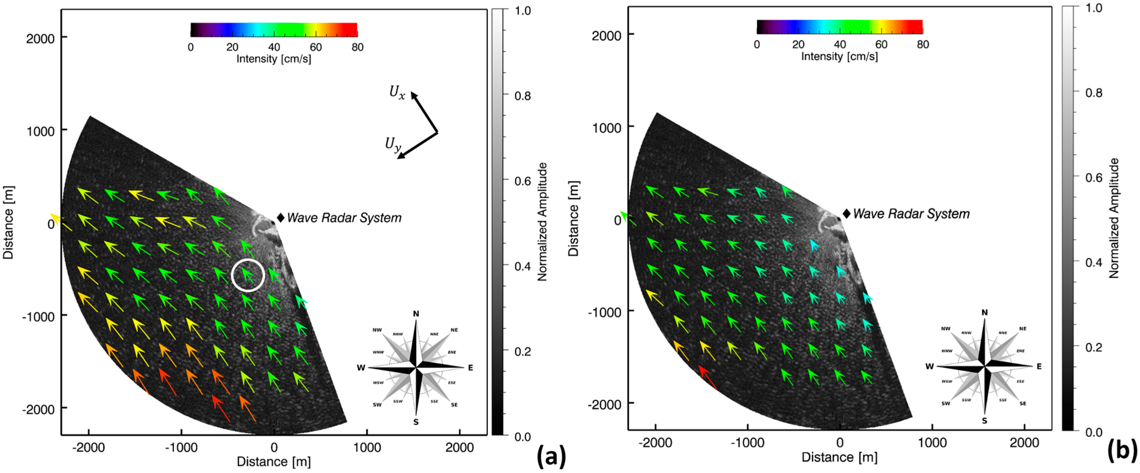
3. Results
4. Discussion
5. Conclusions
Acknowledgments
Author Contributions
Conflicts of Interest
References
- Poulain, P.M.; Bussani, A.; Gerin, R.; Jungwirth, R.; Mauri, E.; Menna, M.; Notarstefano, G. Mediterranean surface currents measured with drifters: From basin to sub inertial scales. Oceanography 2013, 26, 38–47. [Google Scholar] [CrossRef]
- Pazan, S.E. Intercomparison of drogued and undrogued drift buoys. In Proceedings of the MTS/IEEE Oceans’96 Conference, Fort Lauderdale, FL, USA, 3–26 September 1996.
- Paduan, J.D. Wind-Driven motions in the northeast pacific as measured by lagrangian drifters. J. Phys. Oceanogr. 1995, 25, 2819–2830. [Google Scholar] [CrossRef]
- Lumpkin, R.; Pazos, M. Measuring surface currents with SVP drifters: The instrument, its data and some results. In Lagrangian Analysis and Prediction of Coastal and Ocean Dynamics; Griffa, A., Kirwan, J.A.D., Eds.; Cambridge University Press: Cambridge, UK, 2007; pp. 39–67. [Google Scholar]
- Davis, R.E. Drifter observation of coastal currents during CODE: The method and descriptive view. J. Geophys. Res. 1985, 90, 4741–4755. [Google Scholar] [CrossRef]
- Manning, J.P.; McGillicuddy, D.J.; Pettigrewc, N.R.; Churchill, J.H.; Incze, L.S. Drifter observations of the Gulf of Maine Coastal Current. Cont. Shelf Res. 2009, 29, 835–845. [Google Scholar] [CrossRef]
- Petronio, A.; Roman, F.; Nasello, C.; Armenio, V. Large eddy simulation model for wind-driven sea circulation in coastal areas. Nonlinear Process. Geophys. 2013, 20, 1095–1112. [Google Scholar] [CrossRef]
- Nasello, C.; Armenio, V. A new small drifter for shallow water basins: Application to the study of surface currents in the Muggia Bay (Italy). J. Sens. 2016. [Google Scholar] [CrossRef]
- Young, I.R.; Rosenthal, W.; Ziemer, F. A three-dimensional analysis of marine radar images for the determination of ocean wave directionality and surface currents. J. Geophys. Res. 1985, 90, 1049–1059. [Google Scholar] [CrossRef]
- Gangeskar, R. Ocean current estimated from X-band radar sea surface images. IEEE Trans. Geosci. Remote Sens. 2002, 40, 783–792. [Google Scholar] [CrossRef]
- Senet, C.M.; Seemann, J.; Ziemer, F. The near-surface current velocity determined from image sequences of the sea surface. IEEE Trans. Geosci. Remote Sens. 2001, 39, 492–505. [Google Scholar] [CrossRef]
- Senet, C.M.; Seemann, J.; Flampouris, S.; Ziemer, F. Determination of bathymetric and current maps by the method DiSC based on the analysis of nautical X-band radar image sequences of the sea surface (November 2007). IEEE Trans. Geosci. Remote Sens. 2008, 46, 2267–2279. [Google Scholar] [CrossRef]
- Shen, C.; Huang, W.; Gill, E.W.; Carrasco, R.; Horstmann, J. An algorithm for surface current retrieval from X-band marine radar images. Remote Sens. 2015, 7, 7753–7767. [Google Scholar] [CrossRef]
- Serafino, F.; Lugni, C.; Soldovieri, F. A novel strategy for the surface current determination from marine X-band radar data. IEEE Geosci. Remote Sens. Lett. 2010, 7, 231–235. [Google Scholar] [CrossRef]
- Huang, W.; Gill, E. Surface current measurement under low sea state using dual polarized X-band nautical radar. IEEE J. Sel. Top. Appl. Earth Obs. Remote Sens. 2012, 5, 1868–1873. [Google Scholar] [CrossRef]
- Serafino, F.; Lugni, C.; Ludeno, G.; Arturi, D.; Uttieri, M.; Buonocore, B.; Zambianchi, E.; Budillon, G.; Soldovieri, F. REMOCEAN: A flexible X-band radar system for sea-state monitoring and surface current estimation. Geosci. Remote Sens. Lett. 2012, 9, 822–826. [Google Scholar] [CrossRef]
- Plant, W.J.; Keller, W.C. Evidence of Bragg scattering in microwave Doppler spectra of sea return. J. Geophys. Res. 1990, 95, 16299–16310. [Google Scholar] [CrossRef]
- Lee, P.H.Y.; Barter, J.D.; Beach, K.L.; Hindman, C.L.; Lade, B.M.; Rungaldier, H.; Shelton, J.C.; Williams, A.B.; Yee, R.; Yuen, H.C. X-Band microwave Backscattering from ocean waves. J. Geophys. Res. 1995, 100, 2591–2611. [Google Scholar] [CrossRef]
- Wenzel, L.B. Electromagnetic scattering from the sea at low grazing angles. In Surface Waves and Fluxes; Lewis, B.W., Ed.; Kluwer Academic: Norwell, MA, USA, 1990; pp. 41–108. [Google Scholar]
- Ludeno, G.; Reale, F.; Dentale, F.; Pugliese, C.E.; Natale, A.; Soldovieri, F.; Serafino, F. An X-band radar system for bathymetry and wave field analysis in a Harbour area. Sensors 2015, 15, 1691–1707. [Google Scholar] [CrossRef] [PubMed]
- Hessner, K.; Reichert, K.; Borge, J.C.N.; Stevens, C.L.; Smith, M.J. High-resolution X-band radar measurements of currents, bathymetry and sea state in highly inhomogeneous coastal areas. Ocean. Dyn. 2014, 64, 989–998. [Google Scholar] [CrossRef]
- Ludeno, G.; Brandini, C.; Lugni, C.; Arturi, D.; Natale, A.; Soldovieri, F.; Gozzini, B.; Serafino, F. Remocean system for the detection of the reflected waves from the costa concordia ship wreck. IEEE J. Sel. Top. Appl. Earth Obs. Remote Sens. 2014, 7, 3011–3018. [Google Scholar] [CrossRef]
- Ludeno, G.; Flampouris, S.; Lugni, C.; Soldovieri, F.; Serafino, F. A novel approach based on marine radar data analysis for high resolution bathymetry map generation. IEEE Geosci. Remote Sens. Lett. 2014, 11, 234–238. [Google Scholar] [CrossRef]
- Nieto Borge, J.C.; Rodriguez, R.G.; Hessner, K.; Gonzales, I.P. Inversion of marine radar images for surface wave analysis. J. Atmos. Ocean. Technol. 2004, 21, 1291–1300. [Google Scholar] [CrossRef]


| Radar Parameters | Value |
|---|---|
| Antenna rotation period (Δt) | 2.39 s |
| Spatial image spacing (Δx and Δy) | 4.5 m |
| Minimum range | 200 m |
| Maximum range | 2296 m |
| Image number for sequence (Ns) | 32 |
| Antenna height above sea level | ~15 m |
| View angular sector | ~135° |
| Day | Time Survey | Wind Speed (m/s) | Wind Direction (deg) |
|---|---|---|---|
| 15 May 2015 | 12:00 | 4.2 | 176 |
| 15 May 2015 | 13:00 | 7.1 | 155 |
| 15 May 2015 | 14:00 | 5.9 | 177 |
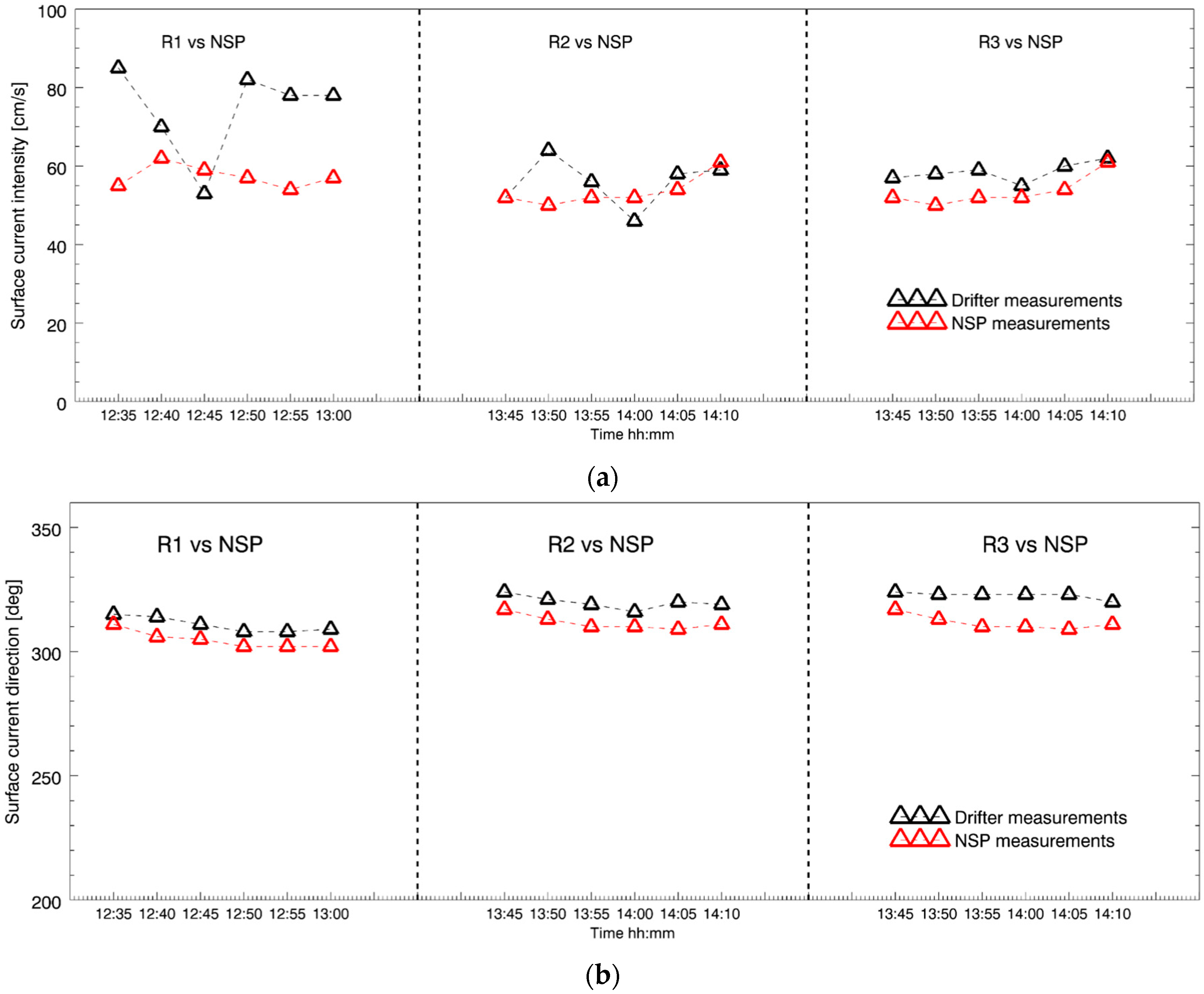
| R1 | |||
|---|---|---|---|
| MeanValues | Std. | Mean Error | |
| UD [cm/s] | 75 | 12 | 30% |
| UR [cm/s] | 57 | 3 | |
| θD [deg] | 311 | 3 | 5% |
| θR [deg] | 305 | 3 | |
| R2 | |||
| MeanValues | Std. | Mean Error | |
| UD [cm/s] | 56 | 6 | 4% |
| UR [cm/s] | 54 | 4 | |
| θD [deg] | 320 | 3 | 6% |
| θR [deg] | 312 | 3 | |
| R3 | |||
| MeanValues | Std. | Mean Error | |
| UD [cm/s] | 59 | 2 | 9% |
| UR [cm/s] | 54 | 4 | |
| θD [deg] | 322 | 1 | 8% |
| θR [deg] | 312 | 3 | |
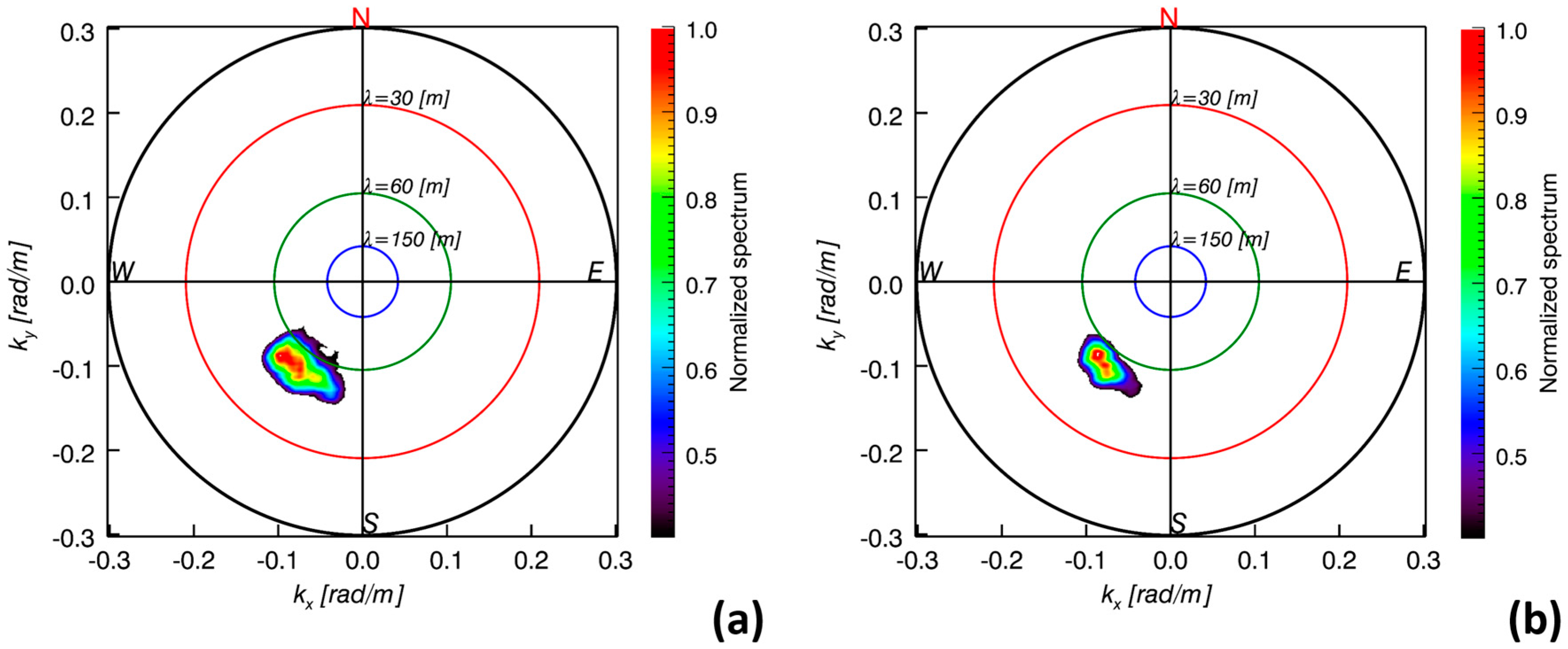
| Time UTC | |||||
|---|---|---|---|---|---|
| 12:40 | 12:50 | 12:55 | 13:45 | 14:05 | |
| Hs [m] | 0.6 | 0.6 | 0.7 | 0.6 | 0.6 |
| Tp [s] | 6.2 | 6.1 | 6.1 | 6.1 | 6.2 |
| λp [m] | 60 | 59 | 59 | 58 | 60 |
| θp [deg] | 215 | 214 | 214 | 215 | 210 |
© 2016 by the authors; licensee MDPI, Basel, Switzerland. This article is an open access article distributed under the terms and conditions of the Creative Commons Attribution (CC-BY) license (http://creativecommons.org/licenses/by/4.0/).
Share and Cite
Ludeno, G.; Nasello, C.; Raffa, F.; Ciraolo, G.; Soldovieri, F.; Serafino, F. A Comparison between Drifter and X-Band Wave Radar for Sea Surface Current Estimation. Remote Sens. 2016, 8, 695. https://doi.org/10.3390/rs8090695
Ludeno G, Nasello C, Raffa F, Ciraolo G, Soldovieri F, Serafino F. A Comparison between Drifter and X-Band Wave Radar for Sea Surface Current Estimation. Remote Sensing. 2016; 8(9):695. https://doi.org/10.3390/rs8090695
Chicago/Turabian StyleLudeno, Giovanni, Carmelo Nasello, Francesco Raffa, Giuseppe Ciraolo, Francesco Soldovieri, and Francesco Serafino. 2016. "A Comparison between Drifter and X-Band Wave Radar for Sea Surface Current Estimation" Remote Sensing 8, no. 9: 695. https://doi.org/10.3390/rs8090695