Supply Chain Cooperation with Price-Sensitive Demand and Environmental Impacts

Abstract

In this paper, we consider a two-echelon sustainable supply chain with price-sensitive demand. The government taxes the carbon footprint of each item caused by producing, transporting, and consuming the products. Both the supplier and retailer can exert efforts to reduce the carbon footprint. In a non-cooperative setting, the government only taxes the supplier, so that the retailer has no incentive to exert any effort to reduce the carbon footprint and the supplier merely decides on the selling price to maximize its own profit. We develop a centralized supply chain and show that there is an optimal solution to maximize the channel profit. Since the centralized policy may not be always not practical, we propose a tax-sharing contract, where both parties profit from the carbon footprint reduction. This problem is modeled as the Stackelberg game and Nash game. The results show that the leader has more power than the follower, which results in more profit. The Stackelberg game provides boundaries for both parties’ profits in the Nash game. Although the tax-sharing contract does not result in full cooperation, its efficiency is still much higher than that of the non-cooperative case. The results are illustrated with some numerical experiments.

1. Introduction

With increased environmental consciousness over the past decade, environmental issues (e.g., global warming, desertification, and acid rain pollution) have become a major concern in industry. Industrial organizations which are involved in sourcing, manufacturing, and transportation should show responsibility towards these problems. However, the typical objectives of most enterprises in a supply chain are to maximize corporate profits and not to reduce pollution. Therefore, the involvement of governments plays a leading role in the environmental protection agenda. Many governments have already enacted green legislation and used financial activities (e.g., green taxation and subsidies) for environmental protection. For example, in 2005, the European Union Emissions Trading System (EU ETS) was launched to reduce greenhouse gas emissions. In 2013, the EU ETS had been operated by more than 11,000 factories, power stations, and other installations in 31 countries (all 28 EU member states plus Iceland, Norway, and Liechtenstein). In September 2013, the European Commission announced a new environmental policy “Communication on Building the Single Market for Green Products”. Its main principle is to evaluate each product’s greenness by one single criterion, known as Product Environmental Footprint (PEF), whose core approach is Life Cycle Assessment (LCA). According to the European Commission, LCA is an internationally-standardized assessment method, which evaluates the environmental burdens and resources consumed along the lifecycle of the product. On the other hand, government intervention, such as taxation and subsidies, can affect the market structure and change the relative market competitiveness, which may even lead to a market reshuffle. To this end, government intervention should be made from a sustainable supply-chain management prospective. The integration of the supply chain has been proved as an effective way to increase the channel profit and efficiency, which could also be the solution to sustainable supply chain management. In this paper, we develop a mathematical model to analyze the eco-efficiency of sustainable supply chains with different cooperation policies under the carbon footprint tax. In the following, we briefly review the relevant literature.

In supply chain management, cooperation is along the supply chain by the coordination between the different parties along the supply chain. Goyal [1] was the first to propose an integrated inventory model with a single-supplier and a single-retailer setting to solve the joint economic lot-sizing problem. Weng [2] used the quantity discount policy to reduce the supplier’s cost and increase the retailer’s demand when the demand is price-sensitive. Huang and Li [3] used game theory to investigate the efficiency of transactions in a manufacturer-retailer co-op advertising supply chain. Viswanathan and Wang [4] proposed quantity discounts and volume discounts as coordination mechanisms in a single-vendor, single-retailer distribution channel with a price-sensitive demand. Sarkar [5] considered a single vendor and single buyer channel coordination mechanism for fixed life products. The vendor required the buyer to change the order quantity and compensated the buyer by offering a quantity discount, so that both players could benefit from coordination.

Recently, with increasing consciousness of environmental protection, the enterprises in supply chains have been putting more effort to implement environmental practices. For this reason, sustainable supply chain management has been studied extensively in the recent literature. Environmental impacts occur through the whole life cycle of a product, from raw material purchasing, to manufacturing, usage, recycling, and disposal. Thus, all of the enterprises in a supply chain should be responsible for pollution control [6]. Sheu et al. [7] proposed a linear multi-objective programming model to manage integrated forward and used-product reverse logistics in a green supply chain. Geldermann et al. [8] used Pinch analysis to study a bicycle company in China, whose objective is to combine different measurements and investigate the overall optimization potential of different process design options. Ferretti et al. [9] developed a model to evaluate the economic and environmental effects of an aluminum supply chain, which examined the concerns about transportation pollution, the manufacturing processes, and recycling. Abdallah et al. [10] proposed a mixed-integer programming model to find the trade-off between costs and respective emissions in a green supply chain. Sarkar et al. [11] developed a three-echelon supply chain with the consideration of transportation and carbon emission cost and the model aimed to reduce the supply chain cost by choosing the best transportation method.

The studies mentioned in the previous paragraph assume that the implementations of environmental practices are in one enterprise or in a cooperative supply chain. However, as the entities in a supply chain may belong to different parties, the crux of the problem lies in the coordination of their activities to enable the implementation of sustainable supply chain management. Effective and efficient cooperation policies need to be developed to tackle this issue. There are several papers that deal with cooperation in sustainable, supply-chain-management settings. Sheu [12] addressed a bargaining framework between producers and reverse-logistics suppliers under government intervention, which seeks equilibrium negotiation solutions for supply chain members. Barari et al. [13] developed a game theoretical model to maximize the producer’s and retailer’s economic profits by leveraging upon the product’s greenness. Ghosh and Shah [14] developed a game theoretical model to analyze how greening levels, prices, and profit are influenced by supply chain structures. Corbett and DeCroix [15] proposed a shared-saving contracts model for chemicals purchasing, which aims to reduce the consumption of indirect materials and maximize the supplier’s and retailer’s profits.

However, these previous studies did not develop mathematical models to analyze the market impacts and eco-efficiency under government intervention in a sustainable supply chain. In this paper, we model cooperation structures in a sustainable supply chain where both parties undertake carbon footprint reduction initiatives, and study the effects of both pricing strategies and government intervention. It is assumed that the government charges a tax on each item’s carbon footprint. Then we analyze the supplier’s and retailer’s reactions in a non-cooperative and a fully cooperative supply chain. As the non-cooperative supply chain is sub-optimal and the fully cooperative supply chain is not always practical, we propose a tax-sharing contract, which can make both parties benefit from a carbon footprint reduction. The numerical experiments are presented to demonstrate the proposed model.

2. Model Formulation for the Sustainable Supply Chain

In this section, we use a mathematical model to analyze the relationship between the profits of the supplier and the retailer and maximize both of their profits. In our setting, the supplier provides a single product to the retailer, who is faced with a price-sensitive demand. The government charges a tax on the carbon footprint of each product, caused by producing, transporting, and consuming the product. With supply chain cooperation, the supplier and retailer both exert effort to reduce the carbon footprint so as to reduce the tax charged by the government.

2.1. Notations and Assumptions

The following assumptions and notations are used through the whole paper. Additional assumptions and notations are introduced when required.

The following notation is used throughout the paper:

p	selling price per unit (decision variable)
c	production cost per unit
t	tax on the carbon footprint per unit
$\beta$	supplier’s margin (the retailer’s margin is $1-\beta$)
$e_s$	effort exerted by supplier to reduce carbon footprint, $0\le e_s\le 1$ (decision variable)
$e_r$	effort exerted by retailer to reduce carbon footprint, $0\le e_r\le 1$ (decision variable)
$z(e_s,e_r)$	carbon footprint per unit ($0\le z(e_s,e_r)\le 1$) with respect to effort $e_s$ and $e_r$
$c_s(e_s)$	supplier’s cost to reduce carbon footprint of each item with respect to effort $e_s$
$c_r(e_r)$	retailer’s cost to reduce carbon footprint of each item with respect to effort $e_r$

Assumptions:

(1)

The inventory is reviewed periodically and the period length is constant.

(2)

The demand (D) in each period is dependent on the selling price (p), which is decided by the retailer, and has a relationship in the form $D=a-bp$.

(3)

The lead time is zero and shortages are not allowed.

(4)

The government charges tax on the carbon footprint of each item.

(5)

The carbon footprint caused by producing, transporting, and consuming the product is a function of the supplier’s and retailer’s effort levels. Without loss of generality, let $z(0,0)=1$. More effort leads to less carbon footprint, i.e., $\partial z(e_s,e_r)/\partial e_s\le 0$, $\partial z(e_s,e_r)/\partial e_r\le 0$. Let $z(e_s,e_r)$ be twice continuously differentiable on [0, 1] × [0, 1]. The returns are decreasing as the effort grows, i.e., ${\partial }^{2}z(e_s,e_r)/{\partial e_s}^2\ge 0$, ${\partial }^{2}z(e_s,e_r)/{\partial e_r}^2\ge 0$. We also assume that $z(e_s,e_r)$ is supermodular in $(e_s,e_r)$, i.e., ${\partial }^{2}z(e_s,e_r)/\partial e_s\partial e_r\ge 0$.

(6)

It costs $c_s(e_s)$ and $c_r(e_r)$ for the supplier and retailer to exert the efforts $e_s$ and $e_r$, respectively. $c_s(e_s)$ and $c_r(e_r)$ are both twice continuously differentiable on [0, 1]. More effort leads to a higher cost, i.e., ${c_s}^{\prime }(e_s)\ge 0$, ${c_r}^{\prime }(e_r)\ge 0$, and both parties’ initial marginal costs of effort are negligible, $c_s^{\prime }(0)=0$ and $c_r^{\prime }(0)=0$. $c_s(e_s)$ and $c_r(e_r)$ are also convex in $e_s$ and $e_r$, respectively, i.e., ${c_s}^{″}(e_s)\ge 0$, ${c_r}^{″}(e_r)\ge 0$. Finally, we assume $\underset{e_s\to 1}{\lim }(c_s^{\prime }(e_s))=\underset{e_r\to 1}{\lim }(c_r^{\prime }(e_r))=\infty$. Although this assumption is not strictly necessary, it can help to define the range of $e_s$ and $e_r$.

(7)

In this research, we focus on both parties’ reactions on carbon footprint tax, but not the distribution of profits. We further assume that without coordination the supplier’s margin is $\beta$. Under the tax-sharing contract, the supplier’s margin is ${\beta }^{\prime }$.

2.2. Decentralized Supply Chain

In general, without cooperation, the government only charges the tax to the supplier. When the two parties of the supply chain make decisions individually, the retailer has no incentive to exert any effort to reduce the carbon footprint. Therefore, $e_r=0$ and $c_r(e_r)=0$.

In such a situation, the retailer’s profit is given by:

$$\begin{array}{ll}{\pi }_r& =(a-bp)(p-c)(1-\beta )-c_r(e_r)(a-bp)\\ & =(a-bp)(p-c)(1-\beta )\end{array}$$

(1)

It can be shown from (1) that ${\partial }^2{\pi }_r/\partial p^2=-2b(1-\beta )<0$, which indicates that ${\pi }_r$ is a concave function of p. By setting $\partial {\pi }_r/\partial p=0$, the optimal price can be obtained and is as follows:

$$p^{*}=\frac{a+bc}{2b}$$

(2)

By substituting $p$ into (1), the optimal retailer’s profit is:

$${{\pi }_r}^{*}=\frac{1}{4}(a-bc)(\frac{a}{b}-c)$$

(3)

In this situation, the supplier’s profit is:

$${\pi }_s=(a-bp)(p-c)\beta -(tz(e_s,e_r)+c_s(e_s))(a-bp)$$

(4)

With $p^{*}=\frac{a+bc}{2b}$ and $e_r=0$, the supplier’s profit becomes:

$${\pi }_s=\frac{1}{4}(a-bc)(a-c)\beta -\frac{1}{2}(tz(e_s,0)+c_s(e_s))(a-bc)$$

(5)

Taking the second partial derivative of ${\pi }_s$ with respect to $e_s$, we get:

$$\frac{{\partial }^2{\pi }_s}{{\partial e_s}^2}=-\frac{1}{2}(a-bc)(t\frac{{\partial }^{2}z(e_s,0)}{{\partial e_s}^2}+{c_s}^{″}(e_s))<0$$

(6)

The optimal $e_s$ can be obtained by setting the first partial derivative of ${\pi }_s$ to zero:

$$\frac{\partial {\pi }_s}{\partial e_s}=-\frac{1}{2}(a-bc)(t\frac{\partial z(e_s,0)}{\partial e_s}+{c_s}^{\prime }(e_s))=0$$

(7)

Since $a-bc>0$, it can be obtained that:

$${c_s}^{\prime }(e_s)=-t\frac{\partial z(e_s,0)}{\partial e_s}$$

(8)

2.3. Centralized Supply Chain

In this section, suppose the supplier and retailer set up a joint company and make decisions together to maximize the channel profit. In this situation, the channel’s profit is given by:

$${\pi }_c={\pi }_s+{\pi }_r=(a-bp)(p-c-tz(e_s,e_r)-c_s(e_s)-c_r(e_r))$$

(9)

First, by taking the second partial derivative of ${\pi }_c$ with respect to p, we get:

$$\frac{{\partial }^2{\pi }_c}{\partial p^2}=-2b<0$$

(10)

Then, by taking the first partial derivative of ${\pi }_c$ with respect to p, we get:

$$\frac{\partial {\pi }_c}{\partial p}=-b(p-c-tz(e_s,e_r)-c_s(e_s)-c_r(e_r))+a-bp$$

(11)

From $\partial {\pi }_c/\partial p=0$, p can be obtained and its value is as follows:

$$p=\frac{c}{2}+\frac{a}{2b}+\frac{1}{2}(tz(e_s,e_r)+c_s(e_s)+c_r(e_r))$$

(12)

Substituting Equation (12) into Equation (9), the channel’s profit becomes:

$${\pi }_c=\frac{1}{4}[a-bc-b(tz(e_s,e_r)+c_s(e_s)+c_r(e_r))](\frac{a}{b}-c-tz(e_s,e_r)-c_s(e_s)-c_r(e_r))$$

(13)

By taking the first derivative of ${\pi }_s$ with respect to $e_s$ and $e_r$, respectively, and setting it to zero, we obtain:

$$\begin{array}{ll}\frac{\partial {\pi }_c}{\partial e_s}& =\frac{1}{4}[a-bc-b(tz(e_s,e_r)+c_s(e_s)+c_r(e_r))](-t\frac{\partial z(e_s,e_r)}{\partial e_s}-{c_s}^{\prime }(e_s))\\ & +\frac{1}{4}(-bt\frac{\partial z(e_s,e_r)}{\partial e_s}-b{c_s}^{\prime }(e_s))(\frac{a}{b}-c-tz(e_s,e_r)-c_s(e_s)-c_r(e_r))=0\end{array}$$

(14)

$$\begin{array}{ll}\frac{\partial {\pi }_c}{\partial e_r}& =\frac{1}{4}[a-bc-b(tz(e_s,e_r)+c_s(e_s)+c_r(e_r))](-t\frac{\partial z(e_s,e_r)}{\partial e_r}-{c_r}^{\prime }(e_r))\\ & +\frac{1}{4}(-bt\frac{\partial z(e_s,e_c)}{\partial e_r}-b{c_r}^{\prime }(e_r))(\frac{a}{b}-c-tz(e_s,e_r)-c_s(e_s)-c_r(e_r))=0\end{array}$$

(15)

From Equations (14) and (15), we obtain necessary conditions for obtaining the maximum ${\pi }_c$:

$${c_s}^{\prime }(e_s)=-t\frac{\partial z(e_s,e_r)}{\partial e_s}$$

(16)

$${c_r}^{\prime }(e_r)=-t\frac{\partial z(e_s,e_r)}{\partial e_r}$$

(17)

By comparing Equations (16) and (17) with Equation (8), we can see that in the decentralized supply chain, the supplier exerts excessive effort and the retailer exerts no effort, which makes the decentralized supply chain inefficient. The centralized supply chain requires that both parties invest a certain proportion to reduce the carbon footprint and then divide the surplus profit reasonably. In practice, it is usually difficult to implement. For this reason, in the next section, we propose a more practically feasible contract.

2.4. Shared-Tax Contract

Since the decentralized supply chain is not efficient and the centralized supply chain is not quite practical, we propose a tax-sharing contract that could make both parties benefit from the carbon footprint reduction. Unlike the centralized supply chain policy, the supplier and the retailer do not engage in a deep collaborative process in the new contract. Under the tax-sharing contract, the supplier requires the retailer to pay a certain proportion of the tax (denoted by ${\beta }^{\prime }$, which is the only component in addition to those in the decentralized supply chain setting), while the retailer could also benefit from the tax breaks. By doing so, the supplier and the retailer could come to an agreement easily. Both parties make a decision according to the proportion of the tax and the other’s choice. So a Nash game and Stackelberg game are used to model the relationship between the profits of the two parties according to their bargaining positions.

Since the retailer should pay a proportion of the carbon footprint tax in the new contract, the retailer requires a higher profit margin $1-{\beta }^{\prime }$ (with ${\beta }^{\prime }<\beta$) than in a decentralized supply chain.

The supplier and retailer’s profit functions are as follows:

$${\pi }_s=(a-bp)(p-c-tz(e_s,e_r)){\beta }^{\prime }-c_s(e_s)(a-bp)$$

(18)

$${\pi }_r=(a-bp)(p-c-tz(e_s,e_r))(1-{\beta }^{\prime })-c_r(e_r)(a-bp)$$

(19)

Since one party’s decision affects the other’s, we use the Stackelberg game and Nash game to get the optimal and equilibrium solutions.

2.4.1. Stackelberg Supplier Game

In this section, we model the relationship between the supplier and the retailer as a non-cooperative Stackelberg game with the supplier as the leader and the retailer as the follower. First, we examine the retailer’s reaction in the second stage.

By taking the second partial derivative of ${\pi }_r$ with respect to p, we have:

$$\frac{{\partial }^2{\pi }_r}{\partial p^2}=-2b(1-{\beta }^{\prime })<0$$

(20)

Since ${\pi }_r$ is concave in p, the optimal price function is determined by:

$$\frac{\partial {\pi }_r}{\partial p}=(1-{\beta }^{\prime })[-b(p-c-tz(e_s,e_r))+a-bp]+b{c}_r(e_r)=0$$

(21)

From Equation (21), we have:

$$p=\frac{a}{2b}+\frac{c}{2}+\frac{1}{2}tz(e_s,e_r)+\frac{c_r(e_r)}{2(1-{\beta }^{\prime })}$$

(22)

Then we consider the retailer’s strategy. By substituting Equation (22) into Equation (19), we have:

$${\pi }_r=\frac{1}{4}(a-bc-btz(e_s,e_r)-\frac{b{c}_r(e_r)}{1-{\beta }^{\prime }})[(\frac{a}{b}-c-tz(e_s,e_r))(1-{\beta }^{\prime })-c_r(e_r)]$$

(23)

By taking the first and second partial derivatives of ${\pi }_r$ with respect to $e_r$, we have:

$$\begin{array}{ll}\frac{\partial {\pi }_r}{\partial e_r}& =\frac{1}{4}(-bt\frac{\partial z(e_s,e_r)}{\partial e_r}-\frac{b{c_r}^{\prime }(e_r)}{1-{\beta }^{\prime }})[(\frac{a}{b}-c-tz(e_s,e_r))(1-{\beta }^{\prime })-c_r(e_r)]\\ & +\frac{1}{4}(a-bc-btz(e_s,e_r)-\frac{b{c}_r(e_r)}{1-{\beta }^{\prime }})[-(1-{\beta }^{\prime })t\frac{\partial z(e_s,e_r)}{\partial e_r}-{c_r}^{\prime }(e_r)]\end{array}$$

(24)

$$\begin{array}{ll}\frac{{\partial }^2{\pi }_r}{{\partial e_r}^2}& =\frac{1}{4}(-bt\frac{{\partial }^{2}z(e_s,e_r)}{{\partial e_r}^2}-\frac{b{c_r}^{″}(e_r)}{1-{\beta }^{\prime }})[(\frac{a}{b}-c-tz(e_s,e_r))(1-{\beta }^{\prime })-c_r(e_r)]\\ & +\frac{1}{4}(-bt\frac{\partial z(e_s,e_r)}{\partial e_r}-\frac{b{c_r}^{\prime }(e_r)}{1-{\beta }^{\prime }})[-(1-{\beta }^{\prime })t\frac{\partial z(e_s,e_r)}{\partial e_r}-{c_r}^{\prime }(e_r)]\\ & +\frac{1}{4}(-bt\frac{\partial z(e_s,e_r)}{\partial e_r}-\frac{b{c_r}^{\prime }(e_r)}{1-{\beta }^{\prime }})[-(1-{\beta }^{\prime })t\frac{\partial z(e_s,e_r)}{\partial e_r}-{c_r}^{\prime }(e_r)]\\ & +\frac{1}{4}(a-bc-btz(e_s,e_r)-\frac{b{c}_r(e_r)}{1-{\beta }^{\prime }})[-(1-{\beta }^{\prime })t\frac{{\partial }^{2}z(e_s,e_r)}{{\partial e_r}^2}-{c_r}^{″}(e_r)]\end{array}$$

(25)

From Equations (24) and (25), we observe that when $\partial {\pi }_r/\partial e_r=0$, ${\partial }^2{\pi }_r/{\partial e_r}^2\le 0$. Therefore, if the optimal $e_r$ is not at the interval boundaries, the necessary condition to maximize ${\pi }_r$ is:

$${c_r}^{\prime }(e_r)=-(1-{\beta }^{\prime })t\frac{\partial z(e_s,e_r)}{\partial e_r}$$

(26)

Thus, the problem becomes:

$$\begin{array}{l}\underset{e_s}{Max}{\pi }_s=(a-bp)(p-c-tz(e_s,e_r)){\beta }^{\prime }-c_s(e_s)(a-bp)\\ s.t.p=\frac{a}{2b}+\frac{c}{2}+\frac{1}{2}tz(e_s,e_r)+\frac{c_r(e_r)}{2(1-{\beta }^{\prime })}\\ {c_r}^{\prime }(e_r)=-(1-{\beta }^{\prime })t\frac{\partial z(e_s,e_r)}{\partial e_r}\\ 0\le e_s\le 1\end{array}$$

(27)

Proposition 1. 

If the manufacturer is the leader and the retailer is the follower, then the following are true:

(i)

The price is negatively correlated to the changes in the supplier’s effort and the retailer’s profit margin.

(ii)

The tax on each item is negatively and positively related to the changes in the carbon footprint and the supplier and retailer’s effort.

(iii)

The retailer’s best response function ${e_r}^{*}(e_s)$ is decreasing in its argument.

Proof. 

For (i), by taking the first partial derivative of p with respect to $e_s$ and $e_r$, it can be found that:

$$\frac{\partial p}{\partial e_s}=\frac{1}{2}t\frac{\partial z(e_s,e_r)}{\partial e_s}<0$$

(28)

$$\frac{\partial p}{\partial e_r}=\frac{1}{2}t\frac{\partial z(e_s,e_r)}{\partial e_r}+\frac{{c_r}^{\prime }(e_r)}{2(1-{\beta }^{\prime })}$$

(29)

From Equations (28) and (29), we finish the proof of (i).

For (ii), it follows directly from Equation (26).

For (iii), by setting the variable ${\tilde{e}}_s=-e_s$. We obtain

$$\begin{array}{l}\frac{{\partial }^2{\pi }_r}{\partial e_r\partial {\tilde{e}}_s}=\frac{1}{4}bt\frac{{\partial }^{2}z(e_s,e_r)}{\partial e_r\partial e_s}[(\frac{a}{b}-c-tz(e_s,e_r))(1-{\beta }^{\prime })-c_r(e_r)]\\ +\frac{1}{4}(-bt\frac{\partial z(e_s,e_r)}{\partial e_r}-\frac{b{c_r}^{\prime }(e_r)}{1-{\beta }^{\prime }})[(1-{\beta }^{\prime })t\frac{\partial z(e_s,e_r)}{\partial e_s}]\\ +\frac{1}{4}bt\frac{\partial z(e_s,e_r)}{\partial e_s}[-(1-{\beta }^{\prime })t\frac{\partial z(e_s,e_r)}{\partial e_r}-{c_r}^{\prime }(e_r)]\\ +\frac{1}{4}(a-bc-btz(e_s,e_r)-\frac{b{c}_r(e_r)}{1-{\beta }^{\prime }})(1-{\beta }^{\prime })t\frac{{\partial }^{2}z(e_s,e_r)}{\partial e_r\partial e_s}\end{array}$$

(30)

We have proved that the necessary condition to maximize ${\pi }_r$ is ${c_r}^{\prime }(e_r)=-(1-{\beta }^{\prime })t\partial z(e_s,e_r)/\partial e_r$ and we have assumed ${\partial }^{2}z(e_s,e_r)/\partial e_s\partial e_r\ge 0$. Therefore, ${\partial }^2{\pi }_r/\partial e_r\partial {\tilde{e}}_s\ge 0$, ${\pi }_r$ is supermodular in $({\tilde{e}}_s,e_r)$. Finally, Theorem 1.2 in Topkis [16] implies the retailer’s best response function ${e_r}^{*}(e_s)$ is decreasing in its argument.

2.4.2. Stackelberg Retailer Game

In practice, some big retailers may dominate the market, which makes retailers more powerful than suppliers. In this section, we assume that the retailer is the leader and the supplier is the follower. First, we talk about the supplier’s reaction in the second stage.

In our setting, the supplier can only decide its effort level $e_s$. By taking the second partial derivative of ${\pi }_s$ with respect to $e_s$:

$$\frac{{\partial }^2{\pi }_s}{{\partial e_s}^2}=-(a-bp)t{\beta }^{\prime }\frac{{\partial }^{2}z(e_s,e_r)}{{\partial e_s}^2}-{c_s}^{″}(e_s)(a-bp)<0$$

(31)

Since ${\pi }_s$ is concave in $e_s$, the supplier’s optimal effort strategy is determined by:

$$\frac{\partial {\pi }_s}{\partial e_s}=-(a-bp)t{\beta }^{\prime }\frac{\partial z(e_s,e_r)}{\partial e_s}-{c_s}^{\prime }(e_s)(a-bp)=0$$

(32)

From Equation (32), we obtain:

$${c_s}^{\prime }(e_s)=-t{\beta }^{\prime }\frac{\partial z(e_s,e_r)}{\partial e_s}$$

(33)

Then, the problem becomes:

$$\begin{array}{l}\underset{p,e_r}{Max}{\pi }_r=(a-bp)(p-c-tz(e_s,e_r))(1-{\beta }^{\prime })-c_r(e_r)(a-bp)\\ s.t.{c_s}^{\prime }(e_s)=-t{\beta }^{\prime }\frac{\partial z(e_s,e_r)}{\partial e_s}\\ 0\le e_r\le 1\\ c\le p\le \frac{a}{b}\end{array}$$

(34)

Proposition 2. 

If the retailer is the leader and the supplier is the follower, then the following are true:

(i)

The supplier’s effort for carbon footprint reduction is positively related to the changes in the tax and the supplier’s profit margin.

(ii)

The supplier’s best response function ${e_s}^{*}(e_r)$ is decreasing in its argument.

Proof. 

For (i), it can be obtained from Equation (33).

For (ii), by setting ${\tilde{e}}_s=-e_s$, we obtain:

$$\frac{{\partial }^2{\pi }_s}{\partial {\tilde{e}}_s\partial e_r}=(a-bp){\beta }^{\prime }t\frac{{\partial }^{2}z(e_s,e_r)}{\partial e_s\partial e_r}$$

(35)

By the assumption that ${\partial }^{2}z(e_s,e_r)/\partial e_s\partial e_r\ge 0$, we prove that ${\partial }^2{\pi }_s/\partial {\tilde{e}}_s\partial e_r\ge 0$ and ${\pi }_r$ is supermodular in $({\tilde{e}}_s,e_r)$. Theorem 1.2 in Topkis [16] establishes (ii).

2.4.3. Nash Equilibrium

In this section, we relax the leader-follower relationship and assume that the two parties have a symmetric relationship. Then, the two parties maximize their profit simultaneously with respect to the other’s strategy. The solution for this game structure is the Nash equilibrium. The problem becomes:

$$\begin{array}{l}\underset{e_s}{Max}{\pi }_s=(a-bp)(p-c-tz(e_s,e_r)){\beta }^{\prime }-c_s(e_s)(a-bp)\\ s.t.0\le e_s\le 1\\ \underset{p,e_r}{Max}{\pi }_r=(a-bp)(p-c-tz(e_s,e_r))(1-{\beta }^{\prime })-c_r(e_r)(a-bp)\\ s.t.0\le e_r\le 1,c\le p\le \frac{a}{b}\end{array}$$

(36)

Proposition 3. 

If the supplier and the retailer have a non-cooperative symmetric relationship, then the following are true:

(i)

The best response function ${e_s}^{*}(e_r)$ and ${e_r}^{*}(e_s)$ are both decreasing in $e_r$ and $e_s$.

(ii)

At least one equilibrium exits in the Nash game.

(iii)

If there are multiple equilibriums, for any two equilibriums $({\widehat{e}}_s,{\widehat{e}}_r)$ and $({\overline{e}}_s,{\overline{e}}_r)$, they can be ordered as ${\widehat{e}}_s\le {\overline{e}}_s$ and ${\widehat{e}}_r\ge {\overline{e}}_r$, or ${\widehat{e}}_s\ge {\overline{e}}_s$ and ${\widehat{e}}_r\le {\overline{e}}_r$. If ${\widehat{e}}_s\le {\overline{e}}_s$ and ${\widehat{e}}_r\ge {\overline{e}}_r$. Finally we have ${\pi }_s({\widehat{e}}_s,{\widehat{e}}_r)\ge {\pi }_s({\overline{e}}_s,{\overline{e}}_r)$ and ${\pi }_r({\widehat{e}}_s,{\widehat{e}}_r)\le {\pi }_r({\overline{e}}_s,{\overline{e}}_r)$.

(iv)

The Stackelberg supplier game offers the upper bounds of the supplier’s profit and the retailer’s effort level, and the lower bounds of the supplier’s effort level and the retailer’s profit. Accordingly, the Stackelberg retailer game offers the upper bounds of the retailer’s profit and the supplier’s effort level, and the lower bounds of the retailer’s effort level and the supplier’s profit.

Proof. 

For (i), it has been proved in Proposition 1 (IV) and Proposition 2 (ii).

For (ii), it follows from Theorem 3.1 in Topkis [16].

For (iii), given two equilibriums $({\widehat{e}}_s,{\widehat{e}}_r)$ and $({\overline{e}}_s,{\overline{e}}_r)$, and ${\widehat{e}}_s\le {\overline{e}}_s$, The retailer’s best response function is decreasing in supplier’s effort and therefore ${\widehat{e}}_r={e_r}^{*}({\widehat{e}}_s)\ge {e_r}^{*}({\overline{e}}_s)={\overline{e}}_r$. Also, ${\pi }_s({\overline{e}}_s,{\overline{e}}_r)\le {\pi }_s({\overline{e}}_s,{\widehat{e}}_r)\le {\pi }_s({e_s}^{*}{({\widehat{e}}_r)}_s,{\widehat{e}}_r)={\pi }_s({\widehat{e}}_s,{\widehat{e}}_r)$ and ${\pi }_r({\widehat{e}}_s,{\widehat{e}}_r)\le {\pi }_r({\overline{e}}_s,{\widehat{e}}_r) \le {\pi }_r({\overline{e}}_s,{e_r}^{*}({\overline{e}}_s))={\pi }_r({\overline{e}}_s,{\overline{e}}_r)$.

For (iv), assume $\underset{\_}{e_s}$ and ${\overline{e}}_r$ are the supplier’s and retailer’s effort levels obtained in the Stackelberg supplier game. If we choose any ${\widehat{e}}_s$ with ${\widehat{e}}_s<\underset{\_}{e_s}$, then the retailer will increase its effort level ${\widehat{e}}_r$, with ${\widehat{e}}_r>{\overline{e}}_r$, according to Equation (26). Since the supplier’s profit is already maximized, with ${\pi }_s(\underset{\_}{e_s},{\overline{e}}_r)>{\pi }_s({\widehat{e}}_s,{\widehat{e}}_r)$, the supplier’s profit will decrease with a lower effort level. From Equation (26), we observe that the retailer will not choose any ${\widehat{e}}_r$ with ${\widehat{e}}_r>{\overline{e}}_r$. The proof is similar for the Stackelberg retailer game.

3. Numerical Experiments

In this section, we carry out numerical experiments to examine both parties’ profits and the carbon footprint under the aforementioned policies. The function of the carbon footprint produced by each item is assumed to be $z(e_s,e_r)={(1-e_s)}^2(1-e_r)$. The supplier’s and retailer’s cost functions to reduce the carbon footprint are assumed to be as follows: $c_s(e_s)={(1-e_s)}^{-3}-3e_s-1$ and $c_r(e_r)={(1-e_r)}^{-3}-3e_r-1$, which have been used in Corbett and DeCroix [3]. We note that these functions satisfy all the conditions that are proposed in the assumption.

For the function of $z(e_s,e_r)$, $c_s(e_s)$ and $c_r(e_r)$ are given, and we can prove that the critical points are local maximums in the centralized supply chain. The proofs are provided in the Appendix A.

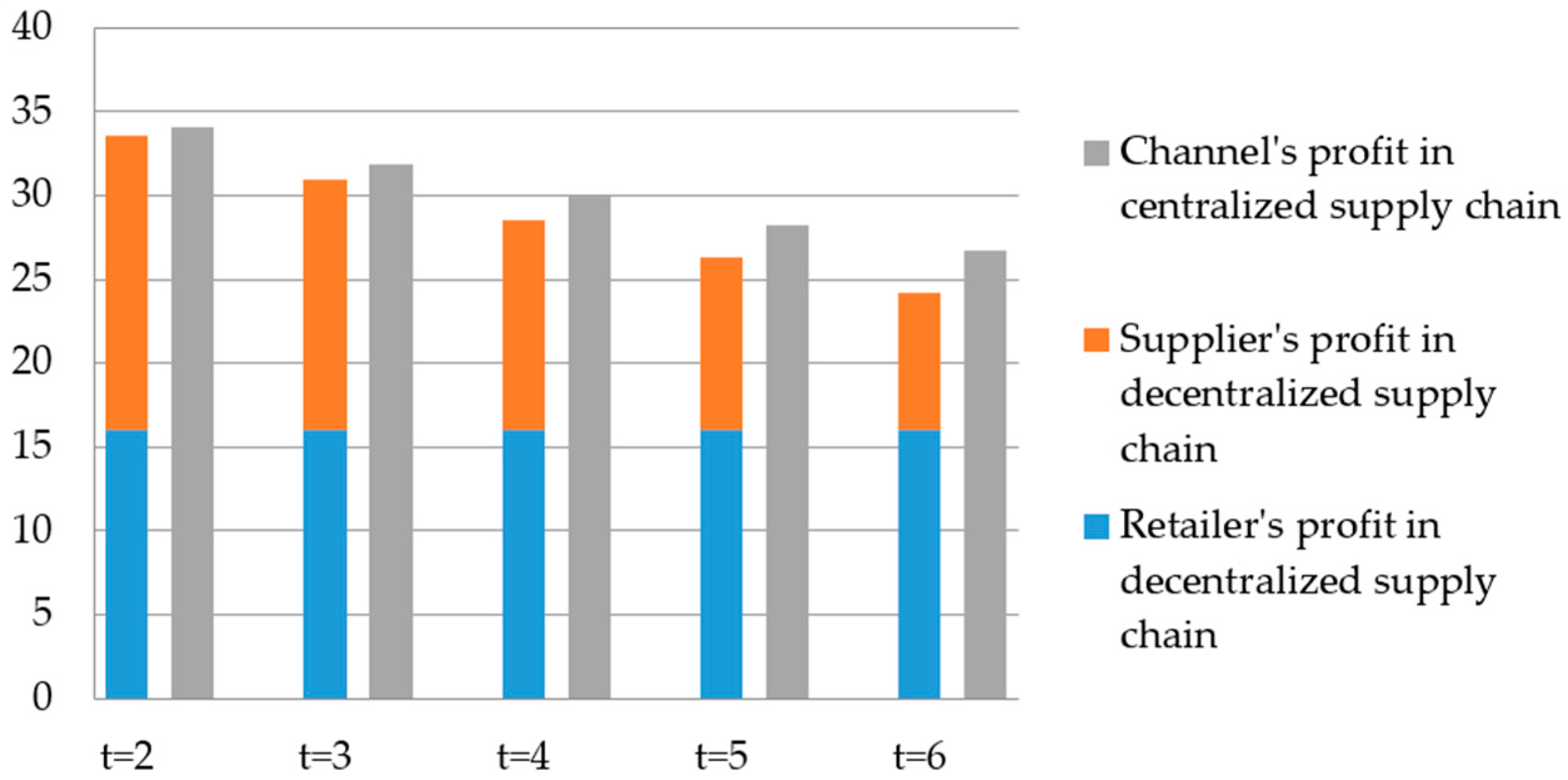
First, we will examine the supplier’s and retailer’s profits under a decentralized and a centralized supply chain with the following values of parameters: $a=10,b=0.4,c=5,\beta =0.6$.

Figure 1 and Figure 2 show that when the tax is only charged to the supplier in a decentralized supply chain, tax changes do not affect the retailer’s decision and profit. The centralized supply chain can both reduce the carbon footprint and increase the channel profit. As the tax increases, cooperation becomes more profitable.

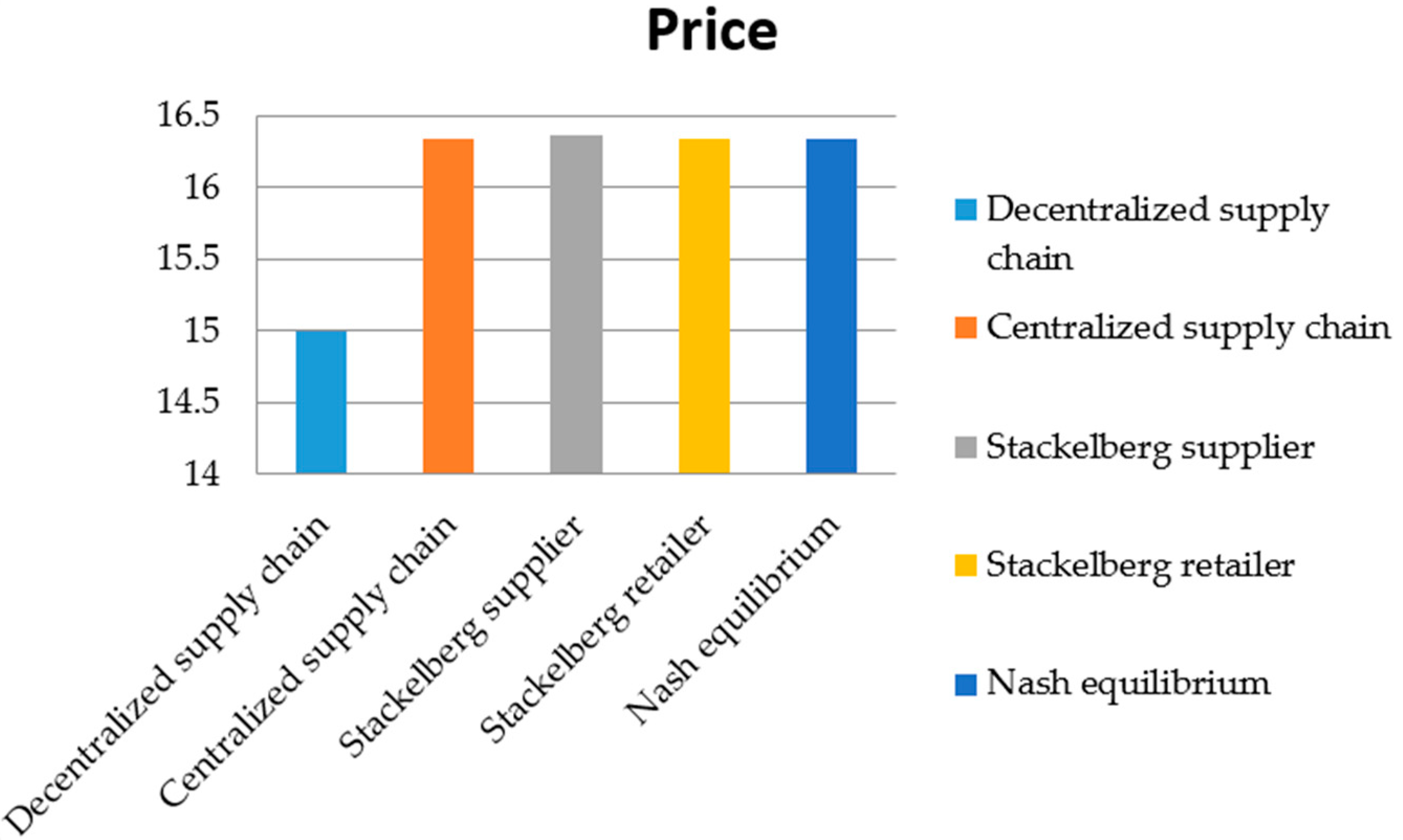
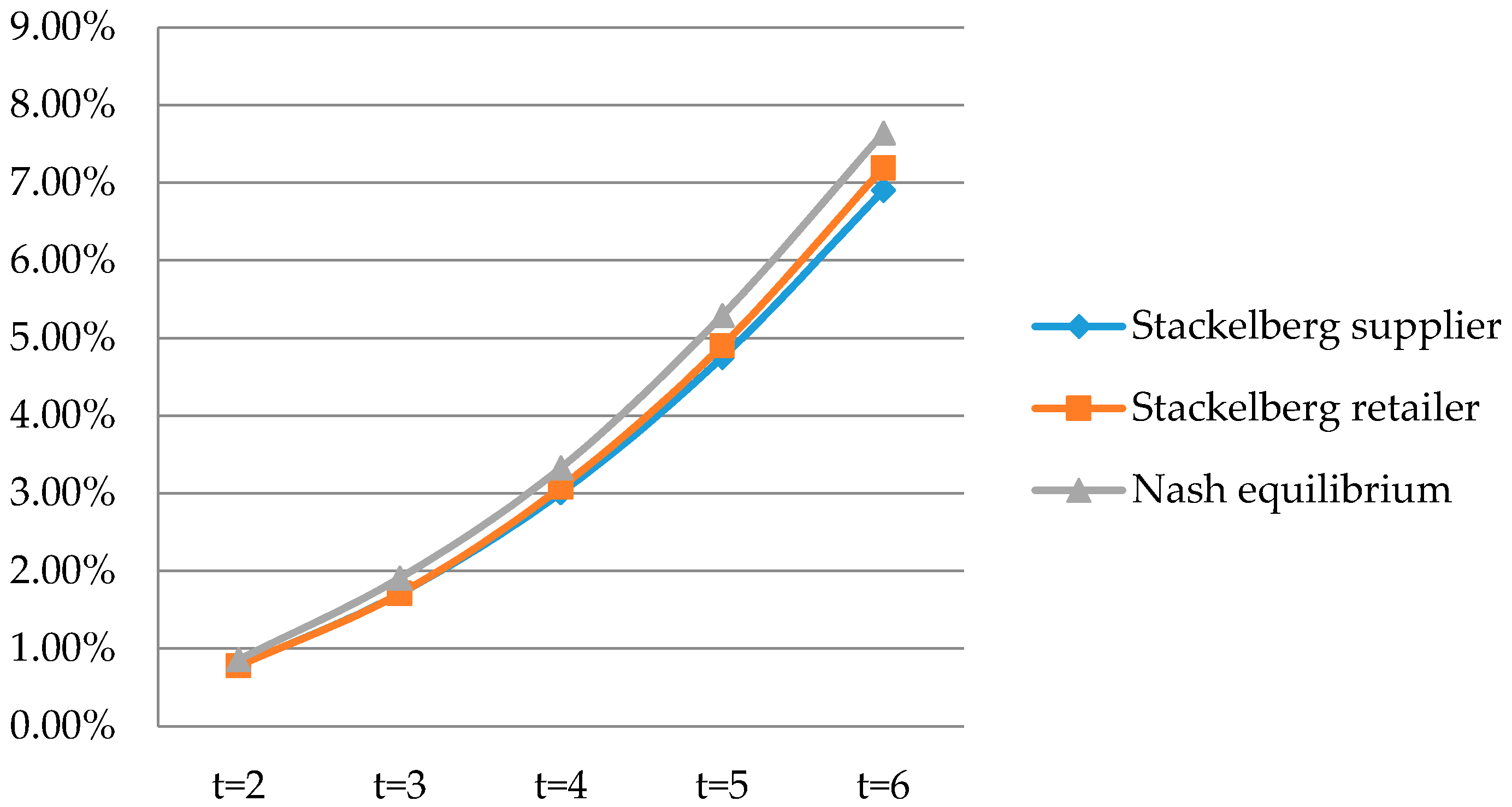
Then we examine the price changes under all the policies, and the supplier’s and retailer’s profits under the Stackelberg and Nash game with the following values of parameters: $a=10,b=0.4,c=5,t=4,{\beta }^{\prime }=0.5,\beta =0.6$. As there are multiple equilibriums in the Nash game, we select the one that produces the largest channel profit.

Figure 3 highlights that when the supplier is the leader, the retailer prefers to set a higher price than the optimal price, and that the price is set lower when the retailer is the leader. This is due to the fact that when the supplier is the leader, less effort is exerted by the supplier. For this reason, the retailer chooses a higher price to earn more profit, and vice versa, which has been proven in Proposition 1 (i). Although the prices are not the same under these policies, the difference is quite small, except in the decentralized supply chain. That is because the price is only dependent on the market demand and production cost, but not affected by the tax. As a result, the price is always lower than the optimal price. The centralized supply chain and tax-sharing contract can limit the size of the market to within a reasonable range and, hence, the total emission of carbon dioxide decreases under these policies. Meanwhile, all of the policies, except the decentralized supply chain, are quite sensitive to the change in tax. 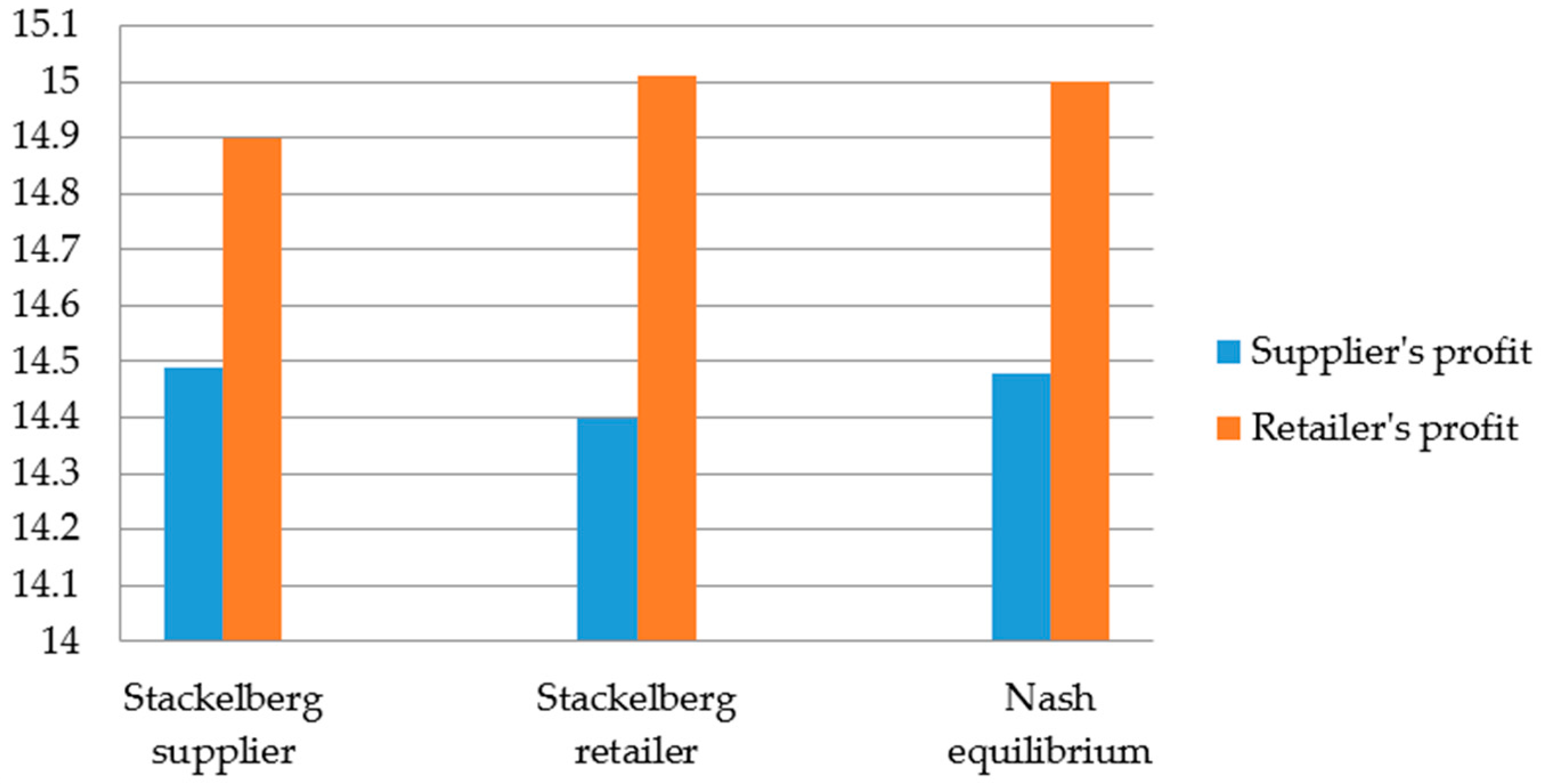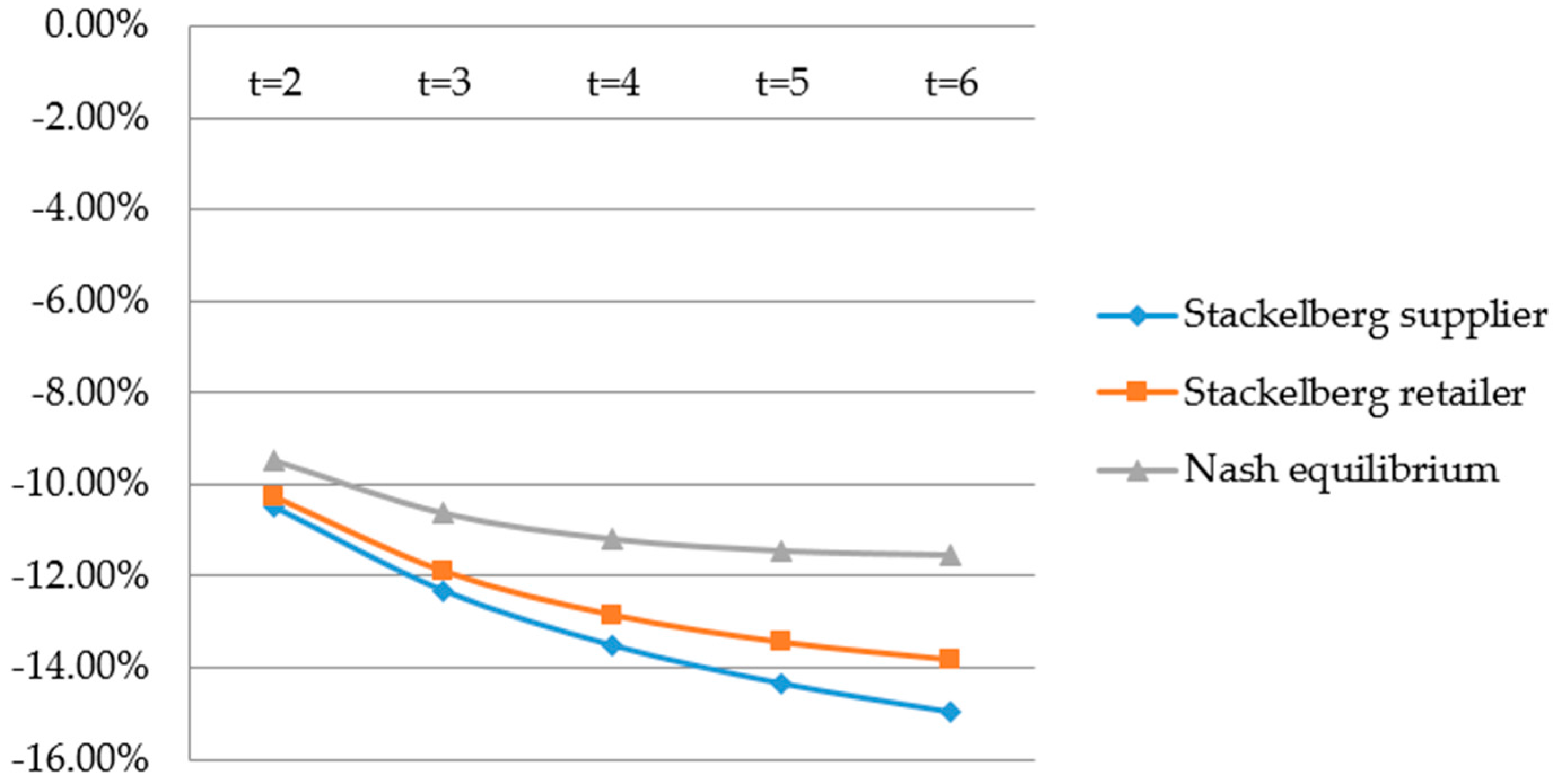From Figure 4 and Figure 5 we observe that the Stackelberg retailer game earns a little more channel profit than the Stackelberg supplier game, because the retailer can decide on the selling price and, thus, have a stronger bargaining power. Therefore, when the retailer is the leader, the supply chain is more efficient. 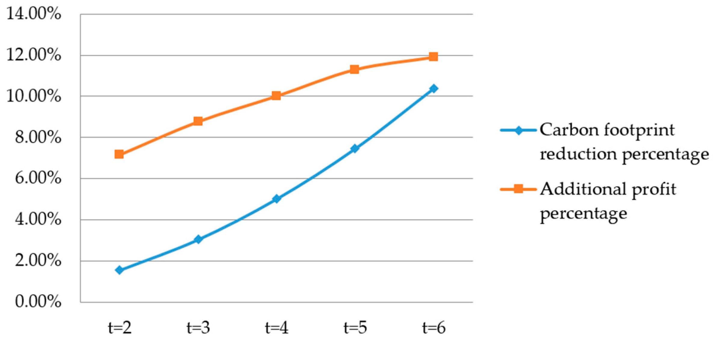Figure 5 and Figure 6 show that the Stackelberg game and Nash game only increase the channel profit, but do not reduce the carbon footprint, compared with the decentralized supply chain. This is because the carbon footprint function is assumed to be $z(e_s,e_r)={(1-e_s)}^2(1-e_r)$, in which the supplier’s effort is more effective. In addition, the tax is only charged to the supplier, so the supplier exerts excessive effort without cooperation. If we assume $z(e_s,e_r)=(1-e_s){(1-e_r)}^2$, then the carbon footprint will decrease under the tax-sharing contract. For this reason, the government should tax the party whose decision could make a more significant reduction in the carbon footprint if there is no cooperation between the supplier and retailer. Even if the carbon footprint is not reduced, the supply chain becomes more efficient under the tax-sharing contract.

4. Conclusions

In this paper, we have studied several cooperation policies in a sustainable supply chain. In a non-cooperative setting, the government only charges tax to the supplier, which provides no incentive for the retailer to reduce the carbon footprint. We also show that a centralized supply chain that can both increase channel profit and reduce the carbon footprint. As the decentralized supply chain is sub-optimal and the centralized supply chain is not always feasible in reality, we proposed a tax-sharing contract. We used the Stackelberg game and Nash game to formulate the relationship between the supplier’s and retailer’s profits. We also found that the Stackelberg game provides the lower and upper bounds of the profits of both parties and effort levels for the Nash game, and that the Stackelberg retailer game is a little more efficient than the Stackelberg supplier game because the retailer can decide on the selling price and has a stronger bargaining power. The distribution of profit is dependent on the relative negotiation power. The decision made by the party who has the higher negotiation power results in a higher profit, which can be shown in the Stackelberg game. Although the tax-sharing contract cannot provide for full cooperation, its channel profit is still higher than in the no-cooperation case.

There are several future extensions from this research. First, we will examine the effect of changing the price-sensitive deterministic demand to stochastic demand. Second, we will also study additional cooperation policies that might increase the channel profit and efficiency. Third, the current model could be extended to the case where multiple suppliers and multiple retailers are involved.